Research digest 4 of 4 · Chapter 10: Failures and stragglers

研究導讀 4 / 4 · 第 10 章：故障與落後者

Resiliency at Scale: Managing Google's TPUv4 Machine Learning Supercomputer大規模的韌性：管理 Google 的 TPUv4 機器學習超級電腦

NSDI 2024Yazhou Zu, Alireza Ghaffarkhah, Hoang-Vu Dang et al. (Google) · paper論文

After reading, you can explain how Google keeps faults away from TPUv4 jobs: placement on any healthy cubes, health checks before and during each job, and routing around a failed optical switch.讀完後，你能說明 Google 如何讓故障遠離 TPUv4 任務：把任務放在任何健康的 cube 上、在任務前與任務中做健康檢查，以及繞過失效的光交換器。

≈ 11 min · 1 interactive panel · 5-question quiz≈ 11 分鐘 · 1 個互動面板 · 5 題測驗Chapter 10 ↗第 10 章 ↗Jump to the quiz ↓跳到測驗 ↓

If you read nothing else

只讀這一段也可以

A TPUv4 supercomputer, or pod, has 4,096 chips in 64 racks called cubes. Each cube is a 4×4×4 block of chips with electrical links inside, and its 96 optical links go to 48 optical circuit switches (OCSes). Training uses compile-time sharding and gang scheduling, so a job runs only if every chip, host and link of its slice is healthy at the same time. This paper describes the software that keeps faults away from running jobs instead of finding them inside the job. The scheduler places a job on any free healthy cubes, and a Pod Manager wires them into the requested torus. Checks before every job and a health daemon on every machine keep faulty parts out. When a whole OCS fails, every cube loses the same link, and routes computed offline detour around it. Measured: with one OCS down, all-to-all throughput stayed at 92.2–101.7% of healthy, and production jobs slowed by 0.5–8.6% per step. Each day, 0.08% of machines, 0.005% of ICI cables and 0.04% of OCSes failed.

一台 TPUv4 超級電腦（pod）有 4,096 顆晶片，分在 64 個稱為 cube 的機櫃中。每個 cube 是 4×4×4 的晶片方塊，內部是電鏈路，它的 96 條光鏈路接到 48 台光路交換器（OCS）。訓練使用編譯期分片與 gang scheduling，所以只有在切片的每顆晶片、每台主機與每條鏈路同時健康時，任務才能執行。這篇論文描述的軟體是讓故障遠離執行中的任務，而不是在任務內部找故障。排程器把任務放在任何空閒且健康的 cube 上，由 Pod Manager 把它們接成所要求的環面。每個任務之前的檢查與每台機器上的健康 daemon 把故障零件擋在外面。當整台 OCS 失效時，每個 cube 都失去同一條鏈路，而離線算好的路由會繞過它。實測：一台 OCS 失效時，all-to-all 吞吐維持在健康時的 92.2–101.7%，生產任務每步變慢 0.5–8.6%。每天有 0.08% 的機器、0.005% 的 ICI 線纜與 0.04% 的 OCS 故障。

1. Where this paper sits1. 這篇論文的位置

Section 10.5 ("Rerouting the torus") uses Google's earlier TPU v4 paper (ISCA 2023) to argue for optical circuit switches with a power law. A fixed slice of $N$ hosts is whole only with probability $a^N$ , where $a$ is the availability of one host. So a fixed 256-host slice at 99.0% host availability is whole only 8% of the time, while a reconfigurable slice needs only enough healthy hosts in a larger pool. That section gives the argument but not the operations: who picks the cubes, who wires them, how faulty parts are kept out, and what happens when an optical switch itself fails. This paper answers those questions from two years of production.

第 10.5 節（「重新接線的環面」）用 Google 較早的 TPU v4 論文（ISCA 2023），以一個次方律支持光路交換器。由 $N$ 台主機組成的固定切片只有在機率 $a^N$ 下是完整的， $a$ 是單台主機的可用性。所以在 99.0% 主機可用性下，固定的 256 主機切片只有 8% 的時間是完整的，而可重構的切片只需要在更大的池子裡有足夠的健康主機。那一節給了論證，卻沒有給營運細節：誰挑 cube、誰接線、故障零件如何被擋在外面，以及光交換器本身故障時會怎樣。這篇論文以兩年的生產經驗回答這些問題。

The other digests of this chapter detect and localize faults inside running GPU jobs, then evict and restart, as in Section 10.4. This paper asks a different question: can the system avoid needing the answer? Its levers are placement at cube granularity, health checks outside the job, and one fault class, the loss of an OCS, that jobs survive without a restart. The torus and OCS basics are in Section 6.9. The fixed routes below contrast with the ECMP hashing of the Chapter 8.

本章其他導讀是在執行中的 GPU 任務內偵測並定位故障，然後逐出並重啟，就像第 10.4 節。這篇論文問的是另一個問題：系統能不能根本不需要這個答案？它的槓桿是以 cube 為單位的配置、任務之外的健康檢查，以及一類任務可以不重啟就撐過的故障：OCS 失效。環面與 OCS 的基礎在第 6.9 節。下面的固定路由則可與第 8 章的 ECMP 雜湊對照。

2. The problem, measured2. 問題，用量測說話

Why ML jobs are fragile. MapReduce-style jobs tolerate a changing set of machines. ML training does not: its sharding is fixed at compile time and all its tasks are gang-scheduled, so every resource must be healthy at once. Google's earlier pods were static: TPUv2 had 256 chips in a 16×16 torus and TPUv3 had 1,024 chips in a 32×32 torus. Static pods have three problems. Maintenance of firmware, links, chips and hosts constantly removes parts. Jobs need contiguous blocks, so the scheduler must preempt smaller jobs to make room. And a pod is usable only after it is fully installed.

為什麼 ML 任務很脆弱。MapReduce 類的任務能容忍機器組合的變動。ML 訓練不能：它的分片在編譯期就固定，所有工作都以 gang scheduling 一起排程，所以每項資源都必須同時健康。Google 較早的 pod 是靜態的：TPUv2 有 256 顆晶片組成 16×16 環面，TPUv3 有 1,024 顆晶片組成 32×32 環面。靜態 pod 有三個問題。韌體、鏈路、晶片與主機的維護不斷拿走零件。任務需要相鄰的區塊，所以排程器必須搶占較小的任務來騰出空間。而一個 pod 要完全裝好才能使用。

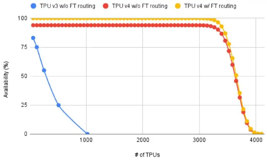
Job availability against job size. The paper's Figure 1 plots measured job availability for deployed TPUv3 static pods and TPUv4 pods. For TPUv3 it falls steeply as jobs approach 1,024 chips. For TPUv4 it stays high, at about 94% without fault-tolerant routing, up to about 50 cubes (3,200 chips), and only then declines, as occasional machine and inter-cube link faults take their toll. The paper also states, without a model, that a 1,024-host job needs 99.9% availability per host in a static design but only 99% with reconfigurable OCSes.

任務可用性對任務大小。論文的 Figure 1 畫出已部署的 TPUv3 靜態 pod 與 TPUv4 pod 實測的任務可用性。TPUv3 的可用性在任務接近 1,024 顆晶片時急劇下降。TPUv4 的可用性一直維持在高點（沒有容錯路由時約 94%），直到約 50 個 cube（3,200 顆晶片）才開始下降，因為偶發的機器與 cube 之間鏈路故障開始產生影響。論文也在沒有給出模型的情況下表示：1,024 台主機的任務在靜態設計下需要每台主機 99.9% 的可用性，有可重構的 OCS 時只需 99%。

Figure 1 of the TPUv4 resiliency paper: availability in percent against number of TPUs for TPU v3 without fault-tolerant routing, TPU v4 without it and TPU v4 with it — Figure 1 of the paper: job availability against job size, which the paper calls measured data from deployed TPUv3 static pods and TPUv4 reconfigurable pods. TPUv3 (blue) falls to zero by 1,024 chips. TPUv4 holds a flat plateau up to about 3,200 chips, about 94% without fault-tolerant routing (red) and close to 100% with it (yellow); both curves fall as the job approaches the whole 4,096-chip pod.論文的 Figure 1：任務可用性對任務大小，論文稱之為來自已部署 TPUv3 靜態 pod 與 TPUv4 可重構 pod 的量測資料。TPUv3（藍）到 1,024 顆晶片就降到零。TPUv4 在約 3,200 顆晶片以內維持平坦的高原：沒有容錯路由時約 94%（紅），有容錯路由時接近 100%（黃）；當任務接近整個 4,096 顆晶片的 pod 時，兩條曲線都會下降。Zu et al., NSDI 2024, Figure 1.

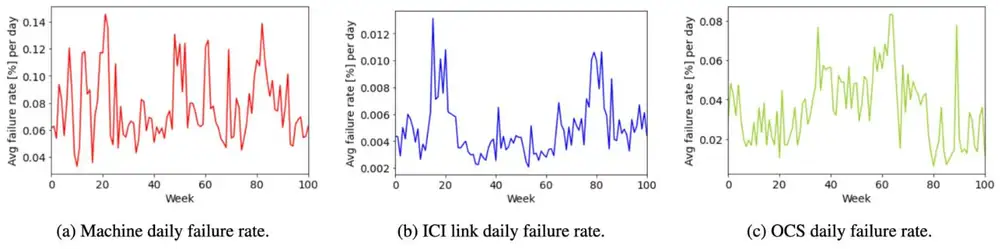
How often parts fail. In an average supercomputer, each day 0.08% of the TPU machines, 0.005% of the ICI cables and 0.04% of the OCSes fail (§5.2). The paper's Figure 12 plots these rates week by week: each point is one week's average daily rate, which is why its caption says "weekly statistics" while the text and the panel titles say daily.

零件多常故障。在一台平均的超級電腦上，每天有 0.08% 的 TPU 機器、0.005% 的 ICI 線纜與 0.04% 的 OCS 故障（§5.2）。論文的 Figure 12 逐週畫出這些故障率：每個點是一週的平均每日故障率，這就是為什麼它的圖說寫「每週統計」，而內文與子圖標題寫每天。

Figure 12 of the TPUv4 resiliency paper: three line charts over 100 weeks of the average daily failure rate in percent of TPU machines, ICI links and OCSes — Figure 12 of the paper: the average daily failure rate of TPU machines, ICI links and OCSes in one supercomputer, one point per week over about 100 weeks (measured). The rates swing from week to week; the averages quoted in the text are 0.08%, 0.005% and 0.04% per day.論文的 Figure 12：一台超級電腦中 TPU 機器、ICI 鏈路與 OCS 的平均每日故障率，約 100 週、每週一個點（實測）。故障率每週起伏；內文引用的平均值是每天 0.08%、0.005% 與 0.04%。Zu et al., NSDI 2024, Figure 12.

Multiplied by the part counts of one pod, and assuming that the cable rate applies to the 6,144 optical links:

乘上一個 pod 的零件數，並假設線纜的故障率適用於 6,144 條光鏈路：

Question問題	Calculation算式	Result結果
Machine failures per pod per day (1,024 machines)每個 pod 每天的機器故障（1,024 台機器）	$1{,}024 \times 0.0008$	$\approx 0.82$
Optical-link failures per pod per day (6,144 links)每個 pod 每天的光鏈路故障（6,144 條鏈路）	$6{,}144 \times 0.00005$	$\approx 0.31$
OCS failures per pod per day (48 OCSes)每個 pod 每天的 OCS 故障（48 台 OCS）	$48 \times 0.0004$	$\approx 0.019$ about 7 per year每年約 7 次

So a pod loses about one machine a day and an OCS a few times a year. The response depends on the blast radius. A failed machine or cable is handled by moving the job to spare healthy cubes. A failed OCS touches every cube in the pod, so moving the job does not help. Jobs route around it instead, and OCS repairs get priority. The panel below shows why spare healthy cubes matter so much for large jobs.

所以一個 pod 大約每天損失一台機器，每年損失幾次 OCS。處理方式取決於影響範圍。機器或線纜故障時，把任務移到備用的健康 cube 上。OCS 故障會牽動 pod 裡的每個 cube，所以搬移任務沒有用。任務改為繞過它，而 OCS 的修復享有優先權。下面的面板說明，為什麼備用的健康 cube 對大型任務如此重要。

Panel 1面板 1

How big a job can the pod place?pod 能放下多大的任務？

Machine availability

a

機器可用性

a

Job size (cubes of 64 chips)任務大小（cube 數，每個 64 顆晶片）

Placement shown on the map地圖上顯示的配置方式

Cube healthy,

c = a^{16}

cube 健康，

c = a^{16}

Healthy cubes on average

平均健康 cube 數

Fixed block works,

a^{16n}

固定區塊可用，

a^{16n}

Any healthy cubes work

任何健康 cube 可用

Largest job placed 95% of days

95% 的日子放得下的最大任務

This sample

這次取樣

Our model, not the paper's. A pod has 64 cubes of 16 machines, and each machine is up with probability $a$ , independently. A cube can join a job only if all 16 of its machines are up, so $c = a^{16}$ . A fixed block needs its own $n$ cubes: $a^{16n}$ . With OCS rewiring, any $n$ healthy cubes will do: $\Pr[\mathrm{Bin}(64, c) \ge n]$ . The map draws one day: red squares are machines that are down, and outlined cubes form the job (red outline: a fixed-block cube that is broken). Defaults: $a = 99.0\%$ , the per-host availability that the paper says suffices with OCSes (versus 99.9% without), and $n = 50$ cubes, about where the paper's measured job availability (its Figure 1) starts to fall. The measured daily failure rate, 0.08% of machines, gives $a \approx 1 - 0.0008 \times$ (days out of service per failure) before planned maintenance; the paper reports no repair times. Try: $a = 99.9\%$ and $n = 64$ ; $a = 99.5\%$ and $n = 32$ with a fixed block.

這是我們的模型，不是論文的。一個 pod 有 64 個 cube，每個 cube 16 台機器，每台機器獨立地以機率 $a$ 正常運作。只有 16 台機器全部正常的 cube 才能加入任務，所以 $c = a^{16}$ 。固定區塊需要它自己的那 $n$ 個 cube： $a^{16n}$ 。有 OCS 重新接線時，任何 $n$ 個健康 cube 都行： $\Pr[\mathrm{Bin}(64, c) \ge n]$ 。地圖畫出某一天：紅色方格是停機的機器，加框的 cube 組成任務（紅框：固定區塊中壞掉的 cube）。預設值： $a = 99.0\%$ ，即論文所說有 OCS 時足夠的每主機可用性（沒有 OCS 時要 99.9%），以及 $n = 50$ 個 cube，大約是論文實測的任務可用性（其 Figure 1）開始下降之處。實測的每日故障率（0.08% 的機器）給出 $a \approx 1 - 0.0008 \times$ （每次故障停機的天數），尚未計入計畫中的維護；論文沒有報告修復時間。試試： $a = 99.9\%$ 且 $n = 64$ ； $a = 99.5\%$ 、 $n = 32$ 並選固定區塊。

3. The design3. 設計

3.1 The life of a job3.1 一個任務的一生

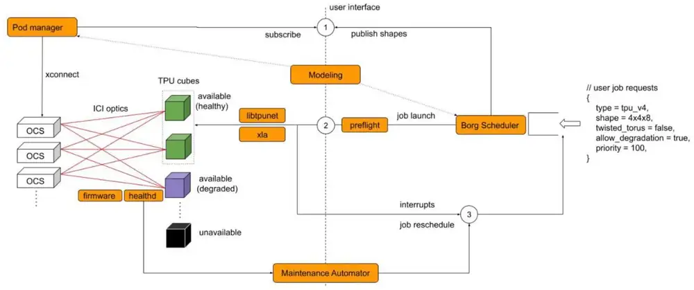
A user asks for a 3D slice shape, for example 4×4×8 chips. The figure below follows the job from the request to training and through the fault loop.

使用者要求一個 3D 切片形狀，例如 4×4×8 顆晶片。下圖追蹤任務從請求到訓練、再經過故障迴圈的過程。

The life of a TPUv4 job. The top row runs once per placement; the preflight check (orange) can send the job back to Borg before it starts. The bottom row is the fault loop: a symptom (red) leads to eviction, rescheduling on other cubes, and repair of the part.一個 TPUv4 任務的一生。上排每次配置執行一次；預檢（橘框）可以在任務開始前把它送回 Borg。下排是故障迴圈：症狀（紅框）導致逐出、在其他 cube 上重新排程，以及零件送修。Drawn for this digest from Zu et al., NSDI 2024, §3 and Figure 5.

Borg, Google's cluster scheduler, queues the job and proposes a set of free cubes; any cubes will do, adjacent or not. The Pod Manager, a replicated service on dedicated network-control servers, polls Borg, rotates the OCS mirrors and confirms. An OCS is a MEMS mirror switch that changes a connection in milliseconds and then holds it as a dedicated optical link. On every machine a borglet agent runs a preflight check; a failure sends the job back to Borg to be placed on other cubes. Then libtpunet, a library inside the job, discovers the topology bottom-up and verifies it with a breadth-first search, assigns chip IDs, and programs the routing tables. It also sizes the link-level flow-control buffers in proportion to each link's round-trip time, synchronizes clocks, and enables each link at both ends together. XLA compiles the program, and training starts. Jobs smaller than a cube need no OCS at all.

Borg（Google 的叢集排程器）把任務排入佇列並提出一組空閒的 cube；任何 cube 都可以，相鄰與否都行。Pod Manager 是在專用網路控制伺服器上的多副本服務，它輪詢 Borg、轉動 OCS 鏡面並回報確認。OCS 是 MEMS 鏡面交換器，能在毫秒內改變連接，之後就保持為一條專用的光鏈路。每台機器上的 borglet 代理執行預檢；失敗就把任務送回 Borg，改放到其他 cube 上。接著任務內的函式庫 libtpunet 由下而上探索拓樸，以廣度優先搜尋驗證，分配晶片 ID，並寫入路由表。它也依每條鏈路的來回時間按比例設定鏈路層流量控制緩衝、同步時鐘，並在兩端同時啟用每條鏈路。XLA 編譯程式後訓練開始。比一個 cube 小的任務完全不需要 OCS。

Wiring cubes into a torus. Each cube exposes 16 links on each of its 6 faces. A link is named {cube, dim, index, polarity}, with index 0–15 and polarity in or out; an OCS is named {dim, index}, 16 OCSes per dimension. Every cube sends its two links of one {dim, index}, one from each opposite face, to the same OCS, so each OCS has 128 cube-facing ports. The cross-connect algorithm (§3.4.1) has four steps. Give each cube in the set a 3D cube coordinate. Compute which cubes are neighbours, with wraparound. Ask each OCS {dim, index} to connect link {dim, index} of each pair of neighbours. Compare with the cached configuration and send only the changes. If a connection is infeasible, the Pod Manager rejects the cube set and Borg proposes another. Twisted tori, whose wraparound links are shifted by an offset, use the same steps with a different neighbour rule.

把 cube 接成環面。每個 cube 的 6 個面各露出 16 條鏈路。鏈路的名稱是 {cube, dim, index, polarity}，index 為 0–15，polarity 為進或出；OCS 的名稱是 {dim, index}，每個維度 16 台。每個 cube 把同一個 {dim, index} 的兩條鏈路（相對兩面各一條）接到同一台 OCS，所以每台 OCS 有 128 個面向 cube 的埠。交叉連接演算法（§3.4.1）有四步。為集合中的每個 cube 指定一個 3D cube 座標。計算哪些 cube 彼此相鄰（含環繞）。要求每台 OCS {dim, index} 連接每對鄰居的 {dim, index} 鏈路。與快取的設定比較，只送出變更。若某條連接無法實現，Pod Manager 就拒絕這組 cube，由 Borg 另提一組。扭轉環面（環繞鏈路平移了一個偏移量）用同樣的步驟，只是鄰居規則不同。

3.2 Health checks outside the job3.2 在任務之外做健康檢查

One database, the datacenter model, holds the racks, cubes, trays, chips, cabling and optics. It is the single source of truth for Borg and the Pod Manager, and every check compares against it. Three mechanisms keep faulty parts out of slices (§3.6):

一個資料庫，也就是資料中心模型，記錄機櫃、cube、托盤、晶片、佈線與光學元件。它是 Borg 與 Pod Manager 唯一的事實來源，每項檢查都與它比對。三個機制把故障零件擋在切片之外（§3.6）：

A preflight check before every job. An end-to-end checker runs a mini sample workload through hardware, driver, firmware and libtpunet. An intent-driven checker compares physical metrics, such as link quality, with "golden" in-spec thresholds. A failure reschedules the job. The paper gives no duration or catch rate.每個任務之前的預檢。端到端檢查器讓一個迷你範例工作負載跑過硬體、驅動程式、韌體與 libtpunet。意圖導向檢查器把鏈路品質等物理指標與「黃金」規格門檻比較。失敗就重新排程。論文沒有給出耗時或攔截率。
healthd on every machine. It watches the machine's 24 unidirectional ICI links, the PCIe channels between TPUs and CPU, and its 4 TPU chips. Symptoms are ranked by severity; a severe one makes healthd tell Borg to evict the job, with notice to checkpoint, and reschedule it. libtpunet stays resident and reports TPU errors, link failures and driver panics through an interrupt.每台機器上的 healthd。它監看機器的 24 條單向 ICI 鏈路、TPU 與 CPU 之間的 PCIe 通道，以及 4 顆 TPU 晶片。症狀依嚴重度分級；嚴重的症狀讓 healthd 通知 Borg 逐出任務（並先通知存檢查點）、再重新排程。libtpunet 常駐，透過中斷回報 TPU 錯誤、鏈路故障與驅動程式當機。
Online link repair. Both ends of a link are repaired together. The Pod Manager first drains the link: a drained link is excluded from user jobs, and its machines still take jobs that avoid it.線上修復鏈路。鏈路兩端協調一起修。Pod Manager 先排空（drain）這條鏈路：被排空的鏈路不給使用者任務使用，而它所在的機器仍可接下避開它的任務。

These checks use fixed thresholds, the method that Minder rejects for GPU fleets because normal values there depend on the task. Here the checked quantities, link quality and firmware state, do not depend on the task, and each slice is owned by one job.

這些檢查使用固定門檻，正是 Minder 在 GPU 機群上拒絕的做法，因為那裡的正常值取決於任務。這裡檢查的量（鏈路品質與韌體狀態）不取決於任務，而且每個切片只屬於一個任務。

3.3 Routing around a missing OCS3.3 繞過失效的 OCS

Fixed routes. libtpunet programs the forwarding tables once, at job start. Each source–destination pair gets one fixed path, chosen offline. On a regular torus the path follows dimension-order routing (DOR): it finishes all hops in one dimension, then the next, in a fixed order, along shortest paths. With two virtual channels, separate buffer classes on each link, DOR cannot deadlock. When a packet must go exactly half way round a ring, it goes the positive way if its source coordinate in that dimension is even and the negative way if odd. In an 8×8×8 torus, a packet from $x = 1$ to $x = 5$ therefore goes X−.

固定路由。libtpunet 只在任務開始時寫入一次轉送表。每一對來源與目的地都得到一條離線選好的固定路徑。在一般環面上，路徑遵循維度順序路由（DOR）：先走完一個維度的所有跳，再走下一個維度，順序固定，且都走最短路徑。有兩個虛擬通道（每條鏈路上分開的緩衝類別）時，DOR 不會死結。當封包必須剛好繞環一半時，若來源在該維度的座標是偶數就走正方向，奇數就走負方向。因此在 8×8×8 環面上，從 $x = 1$ 到 $x = 5$ 的封包走 X−。

What an OCS outage removes. OCS {dim, index} carries link {dim, index} of every cube in the slice. So its loss removes one link from every cube, at the same position in each: a sparse, periodic hole. The figure below shows it for a slice of two cubes.

一次 OCS 失效拿掉什麼。OCS {dim, index} 承載切片中每個 cube 的 {dim, index} 鏈路。所以它失效時，每個 cube 都失去一條鏈路，而且位置相同：一個稀疏、週期性的洞。下圖以兩個 cube 的切片說明。

One plane of constant y in a 4×4×8 slice made of two cubes stacked along z. In each column the X ring has 4 chips, and its wraparound link leaves the cube through an OCS. Columns z and z + 4 use the same OCS, so when OCS B fails, two X links vanish, 4 hops apart along z. Z wraparound links are not drawn.由兩個沿 z 堆疊的 cube 組成的 4×4×8 切片中，y 固定的一個平面。每一欄的 X 環有 4 顆晶片，其環繞鏈路經由一台 OCS 離開 cube。第 z 欄與第 z + 4 欄使用同一台 OCS，所以 OCS B 失效時，兩條 X 鏈路消失，沿 z 相隔 4 跳。圖中未畫 Z 的環繞鏈路。Drawn for this digest from Zu et al., NSDI 2024, §3.4.1, §4.2 and Figure 10.

Wild-first routing. If a pair's DOR path crosses a missing link, the pair uses wild-first routing (WFR): at most one "wild", out-of-order hop per dimension, taken before the normal DOR hops. The sandwich rule says that to avoid a fault in one dimension, hops in another dimension must come before and after it. So yXY avoids X faults (one wild Y hop, then X, then Y), xYX avoids Y faults, and xyZYX avoids single faults in Y and Z. WFR stays deadlock-free with two virtual channels if the order of the wild hops is the reverse of the dimension order: xyZYX is deadlock-free, yxZYX is not. The figure below shows the two-dimensional case.

Wild-first 路由。若某一對的 DOR 路徑經過失效的鏈路，這一對就改用 wild-first 路由（WFR）：每個維度最多一個不照順序的「wild」跳，而且在正常的 DOR 跳之前。三明治規則說：要避開某一維度的故障，必須在它前後都有另一個維度的跳。所以 yXY 避開 X 的故障（先一個 wild Y 跳，再走 X，再走 Y），xYX 避開 Y 的故障，xyZYX 則避開 Y 與 Z 的單一故障。只要 wild 跳的順序與維度順序相反，WFR 用兩個虛擬通道仍不會死結：xyZYX 不會死結，yxZYX 會。下圖是二維的情況。

A piece of a 2D torus with one missing X link (red cross). Route A follows dimension order, X first, and runs into the hole. Routes B and C take one wild Y hop first, then X, then Y back: the X hops are sandwiched between Y hops.二維環面的一部分，少了一條 X 鏈路（紅色叉號）。路徑 A 依維度順序先走 X，撞上缺口。路徑 B 與 C 先走一個 wild Y 跳，再走 X，再走 Y 回來：X 的跳被夾在 Y 的跳之間。Drawn for this digest from Zu et al., NSDI 2024, §4.2 and Figure 11.

Choosing paths offline. An integer linear program picks exactly one path per pair, from the DOR, tie-break and WFR candidates. Its goal is the highest throughput of a traffic pattern, posed as a maximum concurrent flow problem. All-to-all is the main target, with extra constraints so that all-reduce also performs well. A torus looks the same from every chip, so the program solves for one canonical source and translates its paths to every other source. An OCS fault repeats with the cube period, so the canonical fault case is solved once offline, cached, and translated to the actual fault at job setup. The paper gives no solver or solve time. For a regular torus the ideal is easy to bound: losing one of the 16 links per face leaves $15/16 = 93.75\%$ of all-to-all throughput (the paper prints ≈ 93.4%).

離線選路徑。一個整數線性規劃從 DOR、平手規則與 WFR 的候選中，為每一對恰好選一條路徑。它的目標是讓某個流量模式的吞吐最高，寫成最大並行流（maximum concurrent flow）問題。主要目標是 all-to-all，另加限制讓 all-reduce 也表現良好。從每顆晶片看出去，環面都長得一樣，所以只要為一個典型的來源求解，再把路徑平移到其他每個來源。OCS 故障隨 cube 週期重複，所以典型的故障情況只需離線求解一次、快取起來，在任務設定時再平移到實際的故障位置。論文沒有給出求解器或求解時間。一般環面的理想值很容易界定：每面 16 條鏈路失去一條，all-to-all 吞吐剩下 $15/16 = 93.75\%$ （論文印成 ≈ 93.4%）。

4. Implementation4. 實作

The paper describes production services, not a prototype, and gives no code size. Borg runs as a logical Borg Prime backed by replicas, with a borglet on each machine. The Pod Manager runs as one primary plus hot standbys that receive its checkpoints, so it survives crashes and upgrades. Fleet automation handles diagnosis, repair by technicians, and quality checks before repaired hardware returns. Jobs run on TensorFlow, JAX and Pathways with the XLA compiler. The CPUs' datacenter network is managed separately. The system has been in production since 2020. Figure 5 of the paper shows how these services connect.

論文描述的是生產服務而不是原型，也沒有給出程式碼規模。Borg 以多副本支撐的邏輯實例 Borg Prime 運行，每台機器上有一個 borglet。Pod Manager 以一個主實例加上接收其檢查點的熱備援實例運行，所以能撐過當機與升級。機群自動化負責診斷、技術人員維修，以及修好的硬體回歸前的品質檢查。任務在 TensorFlow、JAX 與 Pathways 上執行，使用 XLA 編譯器。CPU 的資料中心網路另外管理。這套系統自 2020 年起在生產環境運行。論文的 Figure 5 顯示這些服務如何相連。

Figure 5 of the TPUv4 resiliency paper: Pod Manager, OCSes, TPU cubes in healthy, degraded and unavailable states, Borg scheduler, preflight, libtpunet, XLA, healthd, firmware and the Maintenance Automator, with numbered steps 1 to 3 — Figure 5 of the paper: how the services connect (a design diagram). Follow the numbers: (1) the Pod Manager and Borg agree on available shapes, (2) Borg launches the job after the preflight check, with libtpunet and XLA bringing up the slice, and (3) on a fault, healthd and firmware report to the Maintenance Automator, which interrupts and reschedules the job. On the right, a user's job request names the slice shape.論文的 Figure 5：各服務如何相連（設計示意圖）。照著編號看：(1) Pod Manager 與 Borg 對可用的形狀取得一致；(2) 通過預檢後 Borg 啟動任務，由 libtpunet 與 XLA 把切片帶起來；(3) 發生故障時，healthd 與韌體回報給 Maintenance Automator，由它中斷任務並重新排程。右側是使用者的任務請求，指定切片形狀。Zu et al., NSDI 2024, Figure 5.

5. What was measured5. 量到了什麼

There is no baseline system. The comparisons are TPUv3 against TPUv4 (Figure 1 of the paper, section 2 above) and a healthy slice against one with an OCS unavailable. Table 2 of the paper measured all-to-all throughput on three slice shapes with all OCSes healthy and with one OCS unavailable. Table 3 measured the step-time slowdown of nine production models while they ran on fault-tolerant routes: six recommendation models (RM), one LLM and two BERT models. The chart below draws both tables.

沒有基準系統。比較的是 TPUv3 對 TPUv4（論文的 Figure 1，見上面第 2 節），以及健康切片對一台 OCS 不可用的切片。論文的 Table 2 量測三種切片形狀在所有 OCS 健康與一台 OCS 不可用時的 all-to-all 吞吐。Table 3 量測九個生產模型在容錯路由上執行時的步時間變慢：六個推薦模型（RM）、一個 LLM 與兩個 BERT 模型。下面的圖畫出這兩張表。

Left: measured all-to-all throughput per slice shape, with all OCSes up and with one OCS down; the orange percentage is the ratio. Right: measured step-time slowdown of nine production workloads on fault-tolerant routes; the six RM models ran on 4×4×8 twisted slices, LLM-1 on 4×4×8, BERT-1 on 4×4×4 and BERT-2 on 4×8×8.左：各切片形狀實測的 all-to-all 吞吐，分為所有 OCS 正常與一台 OCS 失效；橘色百分比是兩者之比（「扭轉」表示扭轉環面）。右：九個生產工作負載在容錯路由上實測的步時間變慢；六個 RM 模型跑在 4×4×8 扭轉切片上，LLM-1 跑在 4×4×8、BERT-1 跑在 4×4×4、BERT-2 跑在 4×8×8。Drawn for this digest from Zu et al., NSDI 2024, Tables 2 and 3.

The regular 4×4×4 torus lost 7.8%, close to the ideal loss of one link in 16 (6.25%). The twisted tori lost almost nothing, and the 4×4×8 twisted slice even gained 1.7%: a twisted torus has several shortest paths, so traffic can shift between dimensions. The gain also shows that the program's objective is only a proxy for real throughput. In production, the paper explains the spread of slowdowns by traffic type. Workloads dominated by all-to-all see little impact, because the optimizer protected all-to-all. All-reduce suffers more: its nearest-neighbour traffic takes a 50% throughput hit on the detours, which better overlap of compute and communication could hide.

一般的 4×4×4 環面損失 7.8%，接近 16 條失去一條的理想損失（6.25%）。扭轉環面幾乎沒有損失，4×4×8 扭轉切片甚至多了 1.7%：扭轉環面有多條最短路徑，流量可以在維度之間移轉。這個增益也說明規劃的目標函數只是實際吞吐的代理。在生產環境中，論文以流量類型解釋變慢幅度的差異。以 all-to-all 為主的工作負載影響很小，因為最佳化器保護了 all-to-all。All-reduce 受害較多：它的最近鄰流量在繞道路由上吞吐損失 50%，更好的計算與通訊重疊可以把它藏起來。

Fleet statistics. Thousands of training jobs are submitted per day, and each pod sees many tens of thousands of OCS cross-connect changes per day (§5.1). 95% of all TPUv4 training jobs opt in to fault-tolerant routing; the rest opt out to avoid nondeterministic performance. Yet over an 8-month window (the paper's Figure 14), fewer than 2% of the jobs were running with it at any time. The paper does not reconcile the two numbers. The likely reading: opting in is a standing choice, and only jobs whose slice meets a current OCS outage use the detours. The share tracked OCS maintenance events; a spike around day 60 came from a planned fleet-wide upgrade of OCS parts.

機群統計。每天有數千個訓練任務提交，每個 pod 每天有好幾萬次 OCS 交叉連接變更（§5.1）。95% 的 TPUv4 訓練任務選擇加入容錯路由；其餘的選擇退出，以避免效能不確定。然而在 8 個月的觀察期間（論文的 Figure 14），任何時刻使用容錯路由執行的任務都不到 2%。論文沒有調和這兩個數字。較可能的解讀是：選擇加入是長期的設定，只有切片碰上當下 OCS 失效的任務才會用到繞道。這個比例隨 OCS 維護事件起伏；第 60 天左右的高峰來自一次計畫中的全機群 OCS 零件升級。

6. Limits and open questions6. 限制與未解的問題

The paper's own future work: lower recovery overhead, higher ICI line rates, randomized routing in the ICI switches to balance load under faults, and hot-standby cubes that receive a job's accelerator state directly, "without ever writing a persistent checkpoint". A careful reader should add:

論文自己的未來工作：降低恢復開銷、提高 ICI 線速、在 ICI 交換器中加入隨機化路由以在故障下平衡負載，以及讓熱備援 cube 直接接收任務的加速器狀態，「完全不寫入持久的檢查點」。細心的讀者還應該補上：

Recovery from a machine fault is still evict, reschedule and restore. The paper gives no checkpoint interval, detection time, restart time, preflight duration or catch rate, so the $D$ , $R$ and $\tau$ of Chapter 10's overhead formula cannot be filled from it.機器故障的恢復仍是逐出、重新排程與還原。論文沒有給出檢查點間隔、偵測時間、重啟時間、預檢耗時或攔截率，所以第 10 章開銷公式中的 $D$ 、 $R$ 與 $\tau$ 無法從這篇論文填入。
The headline availability is a claim, not a measurement we can use. The abstract states 99.98% "system availability" and hardware outages for "~1% of the training jobs". Neither has a definition, a period or a method, so this page reports neither as a result.標題上的可用性是宣稱，不是可用的量測。摘要寫了 99.98% 的「系統可用性」，以及「約 1% 的訓練任務」遇到硬體中斷。兩者都沒有定義、期間或方法，所以本頁不把它們當成結果。
Only one fault class is survived in place. Chip, host and intra-cube link faults still stop the job and move it. The offline program covers one canonical OCS fault; a second fault, or a single bad cable, is drained, and the job is placed elsewhere.只有一類故障能就地撐過。晶片、主機與 cube 內鏈路的故障仍會讓任務停下並搬走。離線規劃只涵蓋一個典型的 OCS 故障；第二個故障或單一條壞線纜會被排空，任務改放到別處。
Monitoring is easier here. Slices are single-tenant, each link retransmits lost packets itself, and the chips report link telemetry. GPU clouds with shared, packet-switched fabrics need the probing of R-Pingmesh and SkeletonHunter.這裡的監控比較容易。切片只有單一租戶，每條鏈路自己重傳遺失的封包，晶片也回報鏈路遙測。共用封包交換網路的 GPU 雲端，則需要 R-Pingmesh 與 SkeletonHunter 那樣的探測。

7. How it connects7. 與其他內容的關聯

Deep dive, section 5: this paper is the operational side of the "Rerouting the torus" paragraph and its $a^N$ argument; the panel above extends that argument to placement on any healthy cubes. Section 1: 0.005% of ICI cables per day is about 0.15% per 30-day month, the same order as HPN's 0.057% of NIC–ToR links per month, for a different kind of link.第 10.5 節：這篇論文是「重新接線的環面」那段及其 $a^N$ 論證的營運面；上面的面板把該論證延伸到放在任何健康 cube 上。第 1 節：每天 0.005% 的 ICI 線纜約等於每 30 天 0.15%，與 HPN 每月 0.057% 的 NIC–ToR 鏈路同一個數量級，只是鏈路種類不同。
Deep dive, section 4: MegaScale detects inside the job and evicts; TPUv4 evicts too, but moves most checks outside the job, into preflight and healthd.第 10.4 節：MegaScale 在任務內偵測並逐出；TPUv4 也會逐出，但把大多數檢查移到任務之外，交給預檢與 healthd。
R-Pingmesh and SkeletonHunter localize faults in shared RoCE fabrics by probing and voting over paths. TPUv4 needs neither tomography nor traffic inference, because each job's routes are fixed and its links are its own.R-Pingmesh 與 SkeletonHunter 在共用的 RoCE 網路中以探測與路徑投票定位故障。TPUv4 既不需要網路斷層掃描，也不需要推測流量，因為每個任務的路由是固定的，鏈路也是它獨占的。
Minder compares machines with each other because GPU "normal" depends on the task; TPUv4's golden thresholds work because link quality does not.Minder 讓機器互相比較，因為 GPU 的「正常」取決於任務；TPUv4 的黃金門檻行得通，因為鏈路品質不取決於任務。
Guided readings: TPU v4 gives the hardware and the goodput curve; Alibaba HPN and Meta RoCE answer the same question in packet-switched fabrics with dual-ToR, backup hosts and uplink headroom. Llama 3 and MegaScale count job interruptions, while this paper counts part failures per day; the two units do not convert directly.論文導讀：TPU v4 提供硬體與 goodput 曲線；Alibaba HPN 與 Meta RoCE 在封包交換網路中用 dual-ToR、備用主機與上行餘裕回答同一個問題。Llama 3 與 MegaScale 計算的是任務中斷，這篇論文計算的是每天的零件故障；兩種單位不能直接換算。
Newer optical designs on this site's reading list (InfiniteHBD, MixNet, Opus) build on the circuit reconfiguration that this paper runs in production.本站閱讀清單上較新的光學設計（InfiniteHBD、MixNet、Opus）都建立在這篇論文於生產環境運行的電路重構之上。

Key numbers關鍵數字

Number	數字	Meaning	意義	Setup
4,096 / 64 / 48	Chips / cubes / OCSes per pod	每個 pod 的晶片 / cube / OCS 數	TPUv4 hardware	TPUv4 硬體
96 / 6,144	Optical ICI links per cube / per pod	每個 cube / 每個 pod 的光 ICI 鏈路	Same	同上
~50 cubes	Job size up to which TPUv4 job availability stays high (3,200 chips)	TPUv4 任務可用性維持高點的任務大小上限（3,200 顆晶片）	Production, Figure 1	生產環境，Figure 1
0.08% / 0.005% / 0.04%	Machines / ICI cables / OCSes failing per day	每天故障的機器 / ICI 線纜 / OCS 比例	Average supercomputer, production	平均的超級電腦，生產環境
92.2% / 101.7% / 98.8%	All-to-all throughput with one OCS down vs healthy: 4×4×4 / 4×4×8 twisted / 4×8×8 twisted	一台 OCS 失效時相對健康的 all-to-all 吞吐：4×4×4 / 4×4×8 扭轉 / 4×8×8 扭轉	Measured on TPUv4 slices	TPUv4 切片實測
0.5–8.6%	Step-time slowdown on fault-tolerant routes	容錯路由下的步時間變慢	Nine production workloads	九個生產工作負載
95% / < 2%	Jobs opted in to fault-tolerant routing / jobs running on it at any time	選擇加入容錯路由的任務 / 任一時刻以它執行的任務	Fleet, 8 months	機群，8 個月
tens of thousands	OCS cross-connect changes per pod per day	每個 pod 每天的 OCS 交叉連接變更	Production	生產環境

Terms used on this page本頁用到的術語

Cube: A rack of 16 TPUv4 machines forming a 4×4×4 block of 64 chips, with electrical links inside.; 16 台 TPUv4 機器組成的機櫃，構成 64 顆晶片的 4×4×4 方塊，內部是電鏈路。
OCS: Optical circuit switch: MEMS mirrors connect one fiber port to another until changed; no packet processing.; 光路交換器：以 MEMS 鏡面把一個光纖埠接到另一個埠，直到改變為止；不處理封包。
ICI: Inter-chip interconnect: Google's direct chip-to-chip network, with per-link retransmission and credit-based flow control.; 晶片間互連：Google 的晶片對晶片直連網路，每條鏈路自行重傳，並以 credit 做流量控制。
Slice切片（slice）: The cubes or chips given to one job, wired as a torus or twisted torus.; 分給一個任務的 cube 或晶片，接成環面或扭轉環面。
healthd: The per-machine daemon that watches links, PCIe and TPU chips and triggers eviction.; 每台機器上監看鏈路、PCIe 與 TPU 晶片並觸發逐出的 daemon。
Preflight check預檢（preflight check）: Tests before every job: a mini workload and comparisons with golden thresholds.; 每個任務之前的測試：一個迷你工作負載，以及與黃金門檻的比較。
Dimension-order routing (DOR)維度順序路由（DOR）: Finish all hops in one dimension, then the next, in a fixed order.; 先走完一個維度的所有跳，再走下一個維度，順序固定。
Wild-first routing (WFR)Wild-first 路由（WFR）: At most one out-of-order hop per dimension, taken before DOR, to detour around a missing link.; 每個維度最多一個不照順序的跳，在 DOR 之前走，用來繞過失效的鏈路。
Virtual channel虛擬通道: A separate buffer class on a link; two of them break the cyclic waits that would deadlock a torus.; 鏈路上分開的緩衝類別；兩個就能打斷會讓環面死結的循環等待。
Maximum concurrent flow最大並行流: An optimization that maximizes the fraction of every demand that can be routed at the same time.; 一種最佳化問題：讓每個需求能同時被路由的比例最大。