Research digest 3 of 5 · Chapter 6: Topology

研究導讀 3 / 5 · 第 6 章：拓樸

MixNet: A Runtime Reconfigurable Optical-Electrical Fabric for Distributed Mixture-of-Experts TrainingMixNet：用於分散式混合專家（MoE）訓練、可在執行期重新配置的光電混合網路

SIGCOMM 2025Xudong Liao, Yijun Sun, Han Tian, …, Zhizhen Zhong, Kai Chen (HKUST, MIT, Peking University, Meta, et al.) · paper論文

After reading, you can explain how MixNet re-wires a regional optical switch inside every MoE layer, why expert compute can hide the switch, and why NIC re-link time is the catch.讀完後，你能說明 MixNet 如何在每個 MoE 層內重新接線區域光交換器、為何專家計算能藏住切換，以及為何 NIC 重新連線時間才是真正的問題。

≈ 11 min · 1 interactive panel · 5-question quiz≈ 11 分鐘 · 1 個互動面板 · 5 題測驗Chapter 6 ↗第 6 章 ↗Jump to the quiz ↓跳到測驗 ↓

If you read nothing else

只讀這一段也可以

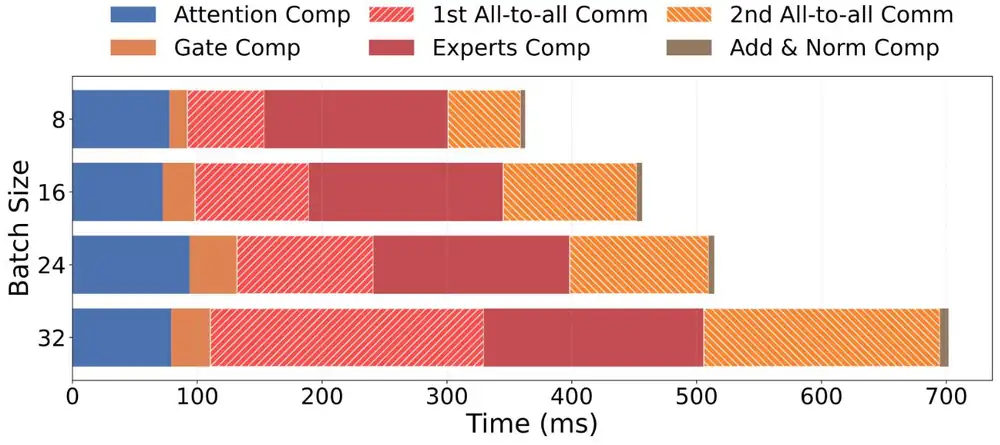
In mixture-of-experts (MoE) training, expert parallelism sends all-to-all bursts whose pattern changes every iteration. On 128 production H800 GPUs training Mixtral 8×7B, they took 33–55% of the iteration time, and only the GPUs of one expert group exchanged them. MixNet keeps a small electrical fat-tree for data and pipeline parallelism and connects most NICs to a regional optical circuit switch (OCS) per expert group. It re-wires that OCS inside every MoE layer, while the experts compute for more than 100 ms. On a 32-A100 prototype with a Polatis OCS, iterations were slightly faster than with four 100G electrical NICs (9.8 s against 11.5 s for Mixtral), but these times exclude the ≈5.7 s that the NICs needed to come back up after each switch.

在混合專家（MoE）訓練中，專家平行會送出 all-to-all 突發流量，模式每次迭代都不同。在 128 顆生產環境 H800 上訓練 Mixtral 8×7B 時，它們占迭代時間的 33–55%，而且只在同一個專家群組的 GPU 之間交換。MixNet 保留小型電子 fat-tree 給資料平行與管線平行，把大部分 NIC 接到每個專家群組一台的區域光電路交換器（OCS）。它在每個 MoE 層內、趁專家計算超過 100 ms 時重新接線這台 OCS。在使用 Polatis OCS 的 32 顆 A100 原型上，迭代比四張 100G 電子 NIC 稍快（Mixtral 為 9.8 s 對 11.5 s），但這些時間不含每次切換後 NIC 重新上線所需的約 5.7 s。

Where this paper sits這篇論文的位置

Section 6.9 showed how TPU v4 sets the mirrors of its optical circuit switches once per job, to join cubes into a torus. Section 3's rail wiring assumes that traffic leaving a server stays on its rail. MoE training breaks both: the router picks experts per token, so the all-to-all matrix changes every iteration and crosses rails. A topology fixed per job (TPU v4, TopoOpt) cannot follow it. Also, a fast OCS has few ports, and a large OCS switches slowly (figure below). No product is both global and fast, so MixNet avoids the need for a global one.

第 6.9 節說明 TPU v4 每個任務只設定一次光電路交換器的鏡面，把 cube 接成環面。第 3 節的 rail 接線則假設離開伺服器的流量留在自己的 rail 上。MoE 訓練兩者都打破：router 依每個 token 挑選專家，所以 all-to-all 矩陣每次迭代都改變，而且會跨 rail。每個任務固定一次的拓樸（TPU v4、TopoOpt）跟不上它。此外，快的 OCS 埠數少，大的 OCS 切換慢（見下圖）。沒有產品同時涵蓋全叢集又夠快，所以 MixNet 設法不需要全域 OCS。

The paper's Table 2 (vendor data) plotted as port count against reconfiguration delay. The green region is the delay one expert computation can hide and the grey line marks about one region's ports, so only the piezo and MEMS switches come close to both. The red line is the delay measured on the authors' Polatis switch, while Google's 2D MEMS, for which no delay is given, is left out.論文 Table 2（廠商資料）畫成埠數對重新配置延遲的圖。綠色區域是一次專家計算能藏住的延遲，灰線標出約一個區域的埠數，因此只有壓電與 MEMS 交換器同時接近兩者。紅線是作者在 Polatis 交換器上量到的延遲，而 Google 的 2D MEMS 因為沒有給出延遲而沒有畫出。Drawn for this digest from Table 2 and Appendix C of the paper; "minutes" is drawn as 1–10 minutes.

The problem, measured問題，用量測說明

The authors profiled Mixtral 8×7B (EP8, TP4, PP4, micro-batch 8) on a DGX SuperPOD with 128 H800 GPUs, 400 Gb/s ConnectX-7 NICs and rail-optimized wiring. Four measured facts drive the design:

作者在一套有 128 顆 H800、400 Gb/s ConnectX-7 NIC 與 rail-optimized 接線的 DGX SuperPOD 上分析 Mixtral 8×7B（EP8、TP4、PP4、micro-batch 8）。驅動設計的是四個量測事實：

Share. The two all-to-alls take 33–55% of the time (42–58% in LLaMA-MoE, up to 68% in Qwen-MoE, Appendix A.1).占比。兩次 all-to-all 占 33–55% 的時間（LLaMA-MoE 為 42–58%，Qwen-MoE 最高 68%，附錄 A.1）。
Bytes. EP carries about 30% of Mixtral's bytes, and more than 80% in LLaMA-MoE and Qwen-MoE (Figure 2).位元組。EP 承載 Mixtral 約 30% 的位元組，在 LLaMA-MoE 與 Qwen-MoE 中超過 80%（Figure 2）。
A window. Expert compute takes more than 100 ms at micro-batch 8, longer than a MEMS or piezo switch (10–25 ms, vendor data).一個窗口。micro-batch 8 時專家計算超過 100 ms，比 MEMS 或壓電交換器的切換（10–25 ms，廠商資料）還長。
Shape. Volumes change between iterations, heavy traffic flows between a few GPU pairs, and all of it stays inside one MoE block's expert group, that is, one pipeline stage (Figures 4–5).形狀。流量在迭代之間變動，大流量只在少數幾對 GPU 之間，而且全部留在一個 MoE 區塊的專家群組內，也就是一個管線階段之內（Figure 4–5）。

Figure 3 of the MixNet paper: horizontal stacked bars of one MoE layer's forward pass for micro-batches 8, 16, 24 and 32, with attention, gate, first all-to-all, expert compute, second all-to-all, and add and norm, on a 0 to 700 ms axis — Figure 3 of the paper, measured in production (Mixtral 8×7B, 128 H800 GPUs, 400 Gb/s): one MoE layer's forward pass for micro-batches 8–32. The hatched bars are the two all-to-alls. Expert compute (dark red) lasts more than 100 ms in every row.論文的 Figure 3，生產環境實測（Mixtral 8×7B、128 顆 H800、400 Gb/s）：micro-batch 8–32 時一個 MoE 層的前向傳遞。斜線條是兩次 all-to-all。每一列的專家計算（深紅）都超過 100 ms。Screenshot of Liao et al., SIGCOMM 2025, Figure 3 (arXiv v4).

The design設計

MixNet matches each parallelism to a fabric (Table 3 of the paper): TP to NVSwitch inside the server, DP and PP to an electrical packet-switched fabric (EPS), and EP to optical circuits.

MixNet 為每種平行方式配一種網路（論文 Table 3）：TP 走伺服器內的 NVSwitch，DP 與 PP 走電子封包交換網路（EPS），EP 走光電路。

1. Two fabrics in every server1. 每台伺服器接兩種網路

Each server splits its NICs: in the paper's simulations 2 of 8 go to an EPS fat-tree and 6 to a regional OCS; the prototype uses 1 and 3 of 4. A server's NIC count on the OCS is its optical degree $\alpha$ . The EPS carries DP and PP, which need cluster-wide reach, plus pairs that get no circuit. The OCS fabric is cut into isolated regions, one per expert group, each with its own controller. A region of about 500 OCS ports holds about 80–250 servers.

每台伺服器把 NIC 分成兩組：論文模擬中 8 張裡 2 張接 EPS fat-tree、6 張接區域 OCS；原型是 4 張中的 1 張與 3 張。一台伺服器接到 OCS 的 NIC 數稱為光學度數 $\alpha$ 。EPS 承載需要觸及全叢集的 DP 與 PP，以及沒分到電路的伺服器對。OCS 網路被切成彼此隔離的區域，每個專家群組一個，各有自己的控制器。一個約 500 埠的區域可容納約 80–250 台伺服器。

The architecture with the simulation default of 8 NICs per server, where 2 NICs (blue) reach the cluster-wide fat-tree and the other 6 (orange) reach their region's OCS. A real region holds tens to hundreds of servers.採模擬預設每台伺服器 8 張 NIC 的架構，其中 2 張（藍）接全叢集的 fat-tree，另外 6 張（橘）接所屬區域的 OCS。實際的區域有數十到數百台伺服器。Drawn for this digest from §4 and Figure 6 of the paper.

2. When to switch: inside the layer2. 何時切換：在層的內部

Each MoE layer runs four all-to-alls per iteration: dispatch sends tokens to their experts and combine brings the results back, in the forward and again in the backward pass. Combine moves the transpose of the dispatch matrix, and backward mirrors forward, so three of the four matrices are known in advance. MixNet re-wires the OCS for combine while the experts compute. The forward dispatch follows the gate directly, so MixNet-Copilot predicts it. It fits a transition matrix $P$ ( $P_{ij}$ : probability that a token sent to expert $i$ in the previous layer goes to expert $j$ here) over the last $k$ iterations:

每個 MoE 層每次迭代有四次 all-to-all：dispatch 把 token 送到專家，combine 把結果送回，前向一次、反向再一次。combine 搬的是 dispatch 矩陣的轉置，反向又與前向對稱，所以四個矩陣中有三個事先已知。MixNet 趁專家計算時為 combine 重新接線。前向 dispatch 緊接在 gate 之後，所以由 MixNet-Copilot 預測。它用最近 $k$ 次迭代擬合轉移矩陣 $P$ （ $P_{ij}$ ：上一層送到專家 $i$ 的 token 在這一層送到專家 $j$ 的機率）：

\min_{P} \; \sum_{i=1}^{k} w_i \,\big\lVert Y_i - P X_i \big\rVert^2

$X_i$ and $Y_i$ are the normalized expert loads of two neighbouring layers, and $w_i$ weights recent iterations. SciPy's SLSQP solver finds $P$ ; the prediction is $P$ times the previous layer's load, so the dispatch switch can run during attention. The text gives no accuracy number. A switch costs nothing when it ends inside its compute window $W$ :

$X_i$ 與 $Y_i$ 是相鄰兩層正規化後的專家負載， $w_i$ 讓近期迭代權重較高。SciPy 的 SLSQP 求解器算出 $P$ ；預測值是 $P$ 乘上一層的負載，所以 dispatch 的切換可以在 attention 期間進行。正文沒有給準確度數字。只要切換在計算窗口 $W$ 內結束，就不花任何時間：

T_{\text{exposed}} = \max\big(0,\; T_{\text{OCS}} + T_{\text{NIC}} - W\big)

One forward MoE layer on a timeline, with step lengths read from Figure 3 and the grey slivers marking the gate and the closing add-and-norm step. Each switch is drawn at the prototype's 46.75 ms mean and ends as its all-to-all starts, while the red bar is the NIC re-link that today's optics add.一個前向 MoE 層的時間線，步驟長度讀自 Figure 3，灰色細條是 gate 與最後的 add-and-norm 步驟。每次切換以原型平均 46.75 ms 畫出，並在對應的 all-to-all 開始時結束，紅條則是現有光模組增加的 NIC 重新連線時間。Drawn for this digest from Figure 3, §5.1 and Appendix C; lengths are approximate chart readings.

3. Which pairs get circuits3. 哪些伺服器對分到電路

Algorithm 1 turns expert loads into a server-to-server demand matrix $D$ , with both directions added because a circuit carries both. With $C_{ij}$ circuits, pair $(i, j)$ needs time $T_{ij} = D_{ij}/C_{ij}$ , and the all-to-all ends with the slowest pair. So the algorithm repeats one step: take the pair with the largest $T_{ij}$ (demand without a circuit counts as infinite) and add a circuit if both servers have a free OCS NIC; otherwise stop. The exact problem is NP-hard; the greedy's run time is not reported. An example with four servers and $\alpha = 3$ (our numbers; ties at infinity go to the larger demand):

Algorithm 1 把專家負載換算成伺服器對伺服器的需求矩陣 $D$ ，兩個方向相加，因為一條電路雙向都能用。有 $C_{ij}$ 條電路時，伺服器對 $(i, j)$ 需要時間 $T_{ij} = D_{ij}/C_{ij}$ ，all-to-all 要等最慢的一對結束。所以演算法重複一步：取 $T_{ij}$ 最大的一對（有需求而無電路視為無限大），若兩台伺服器都有空的 OCS NIC 就加一條電路，否則停止。精確問題是 NP-hard；論文沒有報告貪婪法的執行時間。以下是四台伺服器、 $\alpha = 3$ 的例子（數字是我們設的；同為無限大時先選需求大的）：

Step步驟	Bottleneck pair (largest $T_{ij}$ )瓶頸對（ $T_{ij}$ 最大）	Action動作	Result結果
1	A–B, demand 12, no circuitA–B，需求 12，沒有電路	add a circuit加一條電路	$T_{AB} = 12$
2	C–D, demand 5, no circuitC–D，需求 5，沒有電路	add a circuit加一條電路	$T_{CD} = 5$
3	A–C, demand 2, no circuitA–C，需求 2，沒有電路	add a circuit; A has 1 NIC left加一條電路；A 剩 1 張 NIC	$T_{AC} = 2$
4	A–B at 12A–B，12	add a second circuit; A has none left加第二條電路；A 沒有 NIC 了	$T_{AB} = 12/2 = 6$
5	A–B at 6A–B，6	A has no free NIC: stopA 沒有空的 NIC：停止	slowest pair: 6最慢的一對：6

With one circuit per pair, the slowest pair would need 12: sparse, skewed demand makes a few circuits enough. Uniform demand over many peers would exceed $\alpha$ , and the rest would use the EPS.

如果每一對只有一條電路，最慢的一對需要 12：需求稀疏又偏斜，所以少數電路就夠。若需求平均分散在許多對端，就會超過 $\alpha$ ，其餘流量改走 EPS。

4. Routing over the new circuits4. 在新電路上的路由

For each destination server, a GPU sends through a delegation GPU whose NIC has a direct circuit there (else one on an EPS NIC), gathering data to it over NVSwitch. DP runs as a hierarchical all-reduce on the EPS. With HPN's 0.057% chance that a NIC or link fails during a job, 2 EPS NICs per server both fail with probability below 0.00003%.

對每台目的伺服器，GPU 透過一顆委派 GPU 傳送，它的 NIC 有直達該處的電路（否則選接在 EPS NIC 上的 GPU），資料經 NVSwitch 集中到它。DP 在 EPS 上以階層式 all-reduce 執行。以 HPN 的數據，一個任務期間單一 NIC 或鏈路故障的機率是 0.057%，每台伺服器 2 張 EPS NIC 同時故障的機率低於 0.00003%。

Implementation實作

The prototype has 4 servers, each with 8 A100 GPUs and 4 ConnectX-6 100G NICs (RoCEv2). Per server, three NICs go to a Polatis OCS and one to an NVIDIA SN3700 Ethernet switch: 12 optical and 4 electrical ports. (The production SuperPOD could not be re-cabled because of its warranty.) About 6K lines of C++ hold the topology generator, the OCS controller (TL1 commands) and the runtime; DP and PP use NCCL, EP raw ibverbs, inside Megatron-LM. Only 7 layers of Mixtral 8×7B, 12 of Qwen-MoE and 16 of LLaMA-MoE fit on 32 GPUs.

原型有 4 台伺服器，每台 8 顆 A100 與 4 張 ConnectX-6 100G NIC（RoCEv2）。每台伺服器三張 NIC 接 Polatis OCS、一張接 NVIDIA SN3700 乙太網路交換器：共 12 個光埠與 4 個電埠。（生產環境的 SuperPOD 因保固限制無法重新佈線。）約 6K 行 C++ 包含拓樸產生器、OCS 控制器（TL1 指令）與執行環境；DP 與 PP 用 NCCL，EP 用原生 ibverbs，跑在 Megatron-LM 中。32 顆 GPU 只放得下 Mixtral 8×7B 的 7 層、Qwen-MoE 的 12 層與 LLaMA-MoE 的 16 層。

What was measured量到了什麼

The baseline connects all four 100G NICs of every server to a non-blocking EPS (16 electrical ports) and uses the same parallelization. Figure 10 of the paper compares iteration times:

基準線把每台伺服器的四張 100G NIC 全部接到無阻塞的 EPS（16 個電埠），平行化方式相同。論文 Figure 10 比較迭代時間：

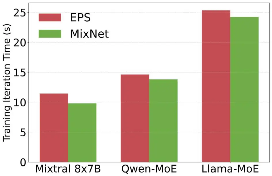
Figure 10 of the MixNet paper: grouped bars of training iteration time for Mixtral 8x7B, Qwen-MoE and Llama-MoE, EPS in red slightly above MixNet in green in each group — Figure 10 of the paper, measured on the 32-A100 prototype with a real Polatis OCS: four electrical NICs (red) against MixNet's one electrical plus three optical NICs (green). MixNet's times exclude the ≈5.7 s NIC re-activation after each switch (Appendix C).論文的 Figure 10，在使用真實 Polatis OCS 的 32 顆 A100 原型上實測：四張電子 NIC（紅）對 MixNet 的一張電子加三張光 NIC（綠）。MixNet 的時間不含每次切換後約 5.7 s 的 NIC 重新啟用（附錄 C）。Screenshot of Liao et al., SIGCOMM 2025, Figure 10 (arXiv v4).

Question (bar heights read from Figure 10)問題（長條高度讀自 Figure 10）	Calculation算式	Result結果
Mixtral 8×7B, 7 layers: EPS 11.5 s, MixNet 9.8 s without NIC re-activationMixtral 8×7B，7 層：EPS 11.5 s，MixNet 9.8 s（不含 NIC 重新啟用）	$11.5 \div 9.8$	$\approx 1.17\times$ MixNet fasterMixNet 較快
Qwen-MoE, 12 layers: 14.6 s against 13.8 s, same exclusionQwen-MoE，12 層：14.6 s 對 13.8 s，同樣不含	$14.6 \div 13.8$	$\approx 1.06\times$
LLaMA-MoE, 16 layers: 25.3 s against 24.2 s, same exclusionLLaMA-MoE，16 層：25.3 s 對 24.2 s，同樣不含	$25.3 \div 24.2$	$\approx 1.05\times$

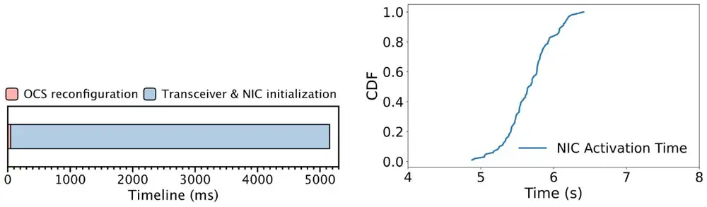
So, without the NIC re-activation, 12 optical plus 4 electrical ports were 5–17% faster than 16 electrical ports; the authors credit circuits for the heavy pairs. Appendix C then timed the switch (figures below): 41.44 ms mean OCS reconfiguration for 1 pair, 42.44 ms for 4 and 46.75 ms for 16, 99% under 70 ms. But the link part of a reconfiguration dominates: the NIC was active again only 5.67 s after the switch on average (p99 6.33 s), and the paper states that its testbed experiments exclude this time.

所以在不計 NIC 重新啟用時，12 個光埠加 4 個電埠比 16 個電埠快 5–17%；作者歸功於把電路分給大流量對。附錄 C 接著量測切換（見下圖）：OCS 重新配置 1 對平均 41.44 ms、4 對 42.44 ms、16 對 46.75 ms，99% 在 70 ms 內。但重新配置中的鏈路部分占了大宗：切換後 NIC 平均 5.67 s 才重新可用（p99 6.33 s），而論文說明測試平台實驗不含這段時間。

Figures 22 and 23 of the MixNet paper: left, a timeline bar to about 5,100 ms that is a thin OCS reconfiguration part followed by transceiver and NIC initialization; right, a CDF of NIC activation time from about 4.9 to 6.4 seconds — Figures 22–23 of the paper (Appendix C, not peer-reviewed), measured on the prototype. Left: one reconfiguration; the OCS part (pink) is a sliver before about 5 s of transceiver and NIC initialization (blue). Right: CDF of the time until the NIC is active, mean 5.67 s.論文的 Figure 22–23（附錄 C，未經同儕審查），原型實測。左：一次重新配置；OCS 部分（粉紅）只是細條，之後是約 5 s 的光模組與 NIC 初始化（藍）。右：NIC 重新可用時間的 CDF，平均 5.67 s。Screenshot of Liao et al., SIGCOMM 2025, Figures 22–23 (arXiv v4).

How much the exclusion hides, as our arithmetic. Appendix B.2 counts two reconfigurations per MoE layer per iteration:

這個排除藏住了多少？以下是我們的計算。附錄 B.2 算每個 MoE 層每次迭代重新配置兩次：

Question (7-layer Mixtral on the prototype)問題（原型上的 7 層 Mixtral）	Calculation算式	Result結果
Switches per iteration每次迭代的切換次數	$7 \times 2$	$14$
OCS time alone, 16-pair mean; each switch fits inside a window of more than 100 ms只算 OCS，16 對的平均；每次切換都放得進超過 100 ms 的窗口	$14 \times 46.75\,\text{ms}$	$\approx 0.65$ scan be hidden可以藏住
NIC time if every switch waited for the link若每次切換都要等鏈路恢復	$14 \times 5.67\,\text{s}$	$\approx 79$ sabout 8× the 9.8 s iteration約為 9.8 s 迭代的 8 倍

Results at 1,024 GPUs and beyond come from packet-level simulation (htsim) and a cost model; we do not report them. The cost case rests on prices: at 400G an OCS port costs $520, an electrical port $1,090 plus a $659 transceiver (Table 4), and the OCS price does not depend on the line rate. Panel 1 lets you vary the switch, the NIC re-link and the window.

1,024 顆 GPU 以上的結果來自封包級模擬（htsim）與成本模型；我們不報告。成本優勢建立在價格上：400G 時一個 OCS 埠 $520，電子埠 $1,090 再加 $659 的光模組（Table 4），而且 OCS 價格與線速無關。面板 1 讓你調整切換、NIC 重新連線與窗口。

Panel 1面板 1

Can the switch hide behind expert compute?切換能藏在專家計算之後嗎？

OCS switch time

T_{\text{OCS}}

OCS 切換時間

T_{\text{OCS}}

NIC re-link

T_{\text{NIC}}

NIC 重新連線

T_{\text{NIC}}

Micro-batch (sets

W

and the all-to-all, Figure 3)micro-batch（決定

W

與 all-to-all，Figure 3）

Switches per MoE layer每個 MoE 層的切換次數

MoE layers

L

MoE 層數

L

Switch time

T_{\text{OCS}} + T_{\text{NIC}}

切換時間

T_{\text{OCS}} + T_{\text{NIC}}

Exposed per switch

每次切換外露

Exposed per iteration

每次迭代外露

Exposed ÷ all-to-all time

外露 ÷ all-to-all 時間

Model: exposed per switch $= \max(0, T_{\text{OCS}} + T_{\text{NIC}} - W)$ ; per iteration it is multiplied by the switches per layer and by $L$ ; the last tile divides it by the iteration's $4L$ all-to-alls. $W$ is the expert compute and the all-to-all is the mean of the two, both read approximately from Figure 3 (production H800, Mixtral 8×7B). Defaults: the prototype's 7-layer Mixtral, the 46.75 ms OCS mean for 16 pairs, and no NIC time, which is how the paper timed its runs. Then pick the measured 5.67 s. The prototype and production numbers come from different machines; combining them is our simplification.

模型：每次切換外露 $= \max(0, T_{\text{OCS}} + T_{\text{NIC}} - W)$ ；每次迭代再乘上每層切換次數與 $L$ ；最後一格除以該迭代 $4L$ 次 all-to-all 的時間。 $W$ 是專家計算時間，all-to-all 取兩次的平均，兩者都是從 Figure 3（生產環境 H800、Mixtral 8×7B）大略讀出的。預設值：原型的 7 層 Mixtral、16 對時 46.75 ms 的 OCS 平均，以及不計 NIC 時間，這正是論文計時的方式。接著選實測的 5.67 s。原型與生產環境的數字來自不同機器；把它們放在一起是我們的簡化。

Limits and open questions限制與未解問題

The NIC, not the mirror. On real hardware, the seconds-long NIC and transceiver re-link, not the optical switch, set the reconfiguration time, and the paper left it out of its timing. Opus found the same with other NICs (about 6 s of firmware link-up, 3 s with auto-negotiation off) and also kept it out of its timing. A transceiver vendor told the authors that this is not fundamental: burst-mode optics for passive optical networks (PON) already re-lock fast, and a Tx/Rx loopback during the switch plus fast-locking clock and data recovery (CDR) would help. Until such optics ship, every switch stalls a region for seconds.問題在 NIC，不在鏡面。在真實硬體上，決定重新配置時間的是長達數秒的 NIC 與光模組重新連線，而不是光交換器，而論文的計時沒有算進去。Opus 用不同的 NIC 也發現同樣的事（韌體約 6 s 才 link-up，關掉自動協商約 3 s），同樣沒有算進它的計時。光模組廠商告訴作者這不是根本限制：被動光網路（PON）用的 burst-mode 光模組早已能快速重新鎖定，切換期間做 Tx/Rx 迴路再加上快速鎖定的時脈資料回復（CDR）也有幫助。在這種光模組上市前，每次切換都會讓一個區域停擺數秒。
Small and truncated. The prototype has 32 GPUs and 7–16 layers per model; the production study is one model on 128 GPUs. Claims at 1,024 GPUs rest on simulation that assumes 25 ms of blocking for the forward dispatch and fully hidden other switches.規模小且模型被截短。原型只有 32 顆 GPU、每個模型 7–16 層；生產環境研究只有 128 顆 GPU 上的一個模型。1,024 顆 GPU 的主張建立在模擬上，模擬假設前向 dispatch 阻塞 25 ms、其他切換完全被藏住。
Locality depends on placement. Regions work because one MoE block's experts sit in one pipeline stage. Expert groups across many servers need larger regions, and $\alpha$ circuits per server cannot reach many peers, so more bytes fall back to the EPS.區域性取決於擺放方式。區域之所以成立，是因為一個 MoE 區塊的專家都在同一個管線階段。跨越許多伺服器的專家群組需要更大的區域，而每台伺服器 $\alpha$ 條電路連不到很多對端，更多位元組會退回 EPS。
Prediction, appendix and prices. The prediction's accuracy appears only as a plot, Appendix C is not peer-reviewed, and the cost case depends on the 400G prices above.預測、附錄與價格。預測準確度只以圖呈現，附錄 C 未經同儕審查，成本優勢取決於上述 400G 價格。

How it connects與其他內容的關聯

TPU v4 sets its OCS once per job; MixNet re-wires twice per MoE layer, at the price of a regional OCS beside an electrical fabric. Against the rail-only paper's premise, EP carries most bytes in fine-grained MoE. Section 3.7 explains dispatch and combine; section 9.4 of the Chapter 4 shows papers that change the all-to-all schedule, while MixNet changes the topology under it. Opus makes each rail one OCS and switches between parallelism phases. ZCube and BST stay static and electrical; Harvest switches a µs-scale photonic fabric inside one collective.

TPU v4 每個任務設定一次 OCS；MixNet 每個 MoE 層重新接線兩次，代價是在電子網路旁加一台區域 OCS。與 rail-only 論文的前提相反，細粒度 MoE 中大多數位元組屬於 EP。第 3.7 節解釋 dispatch 與 combine；第 4 章第 9.4 節介紹改變 all-to-all 排程的論文，而 MixNet 改變的是排程底下的拓樸。Opus 把每條 rail 變成一台 OCS，在平行化階段之間切換。ZCube 與 BST 維持靜態電子網路；Harvest 則在一次集體操作內切換 µs 級的光子網路。

Key numbers關鍵數字

Number數字	What was measured, and where量了什麼、在哪裡量
33–55%	EP all-to-all share of iteration time; Mixtral 8×7B, 128 H800, productionEP all-to-all 占迭代時間的比例；128 顆 H800 上的 Mixtral 8×7B，生產環境
> 100 ms	Expert compute per MoE layer at micro-batch 8; same clustermicro-batch 8 時每個 MoE 層的專家計算；同一叢集
> 80%	EP share of bytes in LLaMA-MoE and Qwen-MoE; profilingLLaMA-MoE 與 Qwen-MoE 中 EP 占位元組的比例；效能分析
11.5 → 9.8 s	Iteration, 7-layer Mixtral, EPS vs MixNet, 32-A100 prototype, excluding NIC re-activation迭代時間，7 層 Mixtral，32 顆 A100 原型上 EPS 對 MixNet，不含 NIC 重新啟用
14.6 → 13.8 s · 25.3 → 24.2 s	Qwen-MoE (12 layers), LLaMA-MoE (16 layers), same exclusionQwen-MoE（12 層）與 LLaMA-MoE（16 層）的相同比較，同樣不含
41.44 / 42.44 / 46.75 ms	Mean OCS reconfiguration for 1 / 4 / 16 pairs; 99% under 70 ms; prototype1／4／16 對時 OCS 的平均重新配置時間；99% 在 70 ms 內；原型
5.67 s (p99 6.33 s)	Time until the NIC is active again after a switch; prototype切換後 NIC 重新可用的時間；原型
≈ 6K lines	C++ for controller and runtime控制器與執行環境的 C++ 程式

Terms used on this page本頁用到的術語

Optical circuit switch (OCS): A switch that connects fibers with mirrors; it reads no packets.; 以鏡面連接光纖的交換器；不讀封包。
EPS: Electrical packet switching: an Ethernet or InfiniBand fabric.; 電子封包交換：乙太網路或 InfiniBand 網路。
Dispatch / combine: The two all-to-alls of an MoE layer: tokens to experts, results back.; MoE 層的兩次 all-to-all：把 token 送到專家，再把結果送回來。
Optical degree $\alpha$: The number of a server's NICs attached to the OCS.; 一台伺服器接到 OCS 的 NIC 數。
Region: An isolated slice of the OCS fabric for one expert group, with its own controller.; OCS 網路中供一個專家群組使用、彼此隔離的一塊，有自己的控制器。
MixNet-Copilot: The predictor of the forward dispatch.; 預測前向 dispatch 的元件。
Delegation GPU: The GPU whose NIC carries a server's traffic toward one destination server.; 其 NIC 負責把本伺服器流量送往某一台目的伺服器的 GPU。
Burst-mode transceiver / CDR: Optics that re-lock fast after the signal stops; CDR is the receiver circuit that must re-lock.; 訊號中斷後能快速重新鎖定的光模組；CDR 是接收端必須重新鎖定的電路。