Failures and stragglers: the arithmetic of staying up故障與落後者:保持運轉的算術
Learn how often the parts of a large cluster fail, why one failure stops the whole job, how often to checkpoint, how recovery is automated, how network design makes failures cheaper, and why the slowest rank sets the pace even when nothing fails.了解大型叢集的零件多常故障、為何一次故障會讓整個任務停下、多久做一次檢查點、恢復如何自動化、網路設計如何讓故障的代價變小,以及為何即使沒有故障,最慢的 rank 仍決定節奏。
This chapter builds on Chapters 1, 4, 6, 9. These earlier terms appear most often below; each chip links to its definition.
New terms in this chapter (7)本章新名詞(7)
Each term is defined in the text where it first appears; the link jumps there. Terms from earlier chapters are listed under "Before you start".
每個名詞都在它第一次出現的段落中定義,點連結可跳過去。前面各章的名詞列在「開始之前」。
- Silent data corruption (SDC)靜默資料損毀(SDC) A GPU that produces wrong results without raising an error. GPU 產生錯誤結果卻不報錯。
- MTBFMTBF(平均故障間隔) Mean time between failures; for a job that stops when any part fails, the failure rates of all parts add. 平均故障間隔;若任一零件故障就停機,所有零件的故障率相加。
- Watchdog, heartbeat看門狗(watchdog)、心跳 Timers and periodic status messages that detect a hung or dead rank. 偵測卡住或失效 rank 的計時器與定期狀態訊息。
- Effective training time有效訓練時間 The share of wall-clock time in which the job makes progress that it keeps. 工作在牆鐘時間中產生可保留之進度的比例。
- Young–Daly intervalYoung–Daly 間隔 The checkpoint interval that minimizes lost time: about √(2 × checkpoint pause × MTBF). 使損失時間最小的檢查點間隔:約 √(2 × 檢查點暫停 × MTBF)。
- Standby pool, spare備用池、備援 Spare machines kept ready so a failed one can be replaced without waiting for a repair. 預備的備用機器,故障時可立即替換,不必等待修理。
- Jitter, order statistics抖動、順序統計 Random step-to-step variation of each rank; the step waits for the maximum, which grows with the number of ranks. 每個 rank 每步的隨機變動;步驟等待最大值,而最大值隨 rank 數成長。
10.1What fails, and how often什麼會壞,多常壞
Mechanism. In the language of reliability engineering, every part of a synchronous training job is in series. The job works only if every GPU, every NIC, every link, every switch and every process works. A series system fails at the sum of its parts' failure rates. That is why the question is never "how reliable is one GPU" but "how many parts are there, and what is the sum". The Llama 3 paper gives the only public table of what actually stopped a 16K-GPU run (Llama 3 §3.3.4, Table 5). It is reproduced here with the paper's own counts and percentages.
機制。用可靠度工程的語言來說,同步訓練任務的每個零件都是串聯的。只有當每顆 GPU、每張 NIC、每條鏈路、每台交換器與每個行程都正常,任務才能運作。串聯系統的故障率是各零件故障率的總和。所以問題從來不是「一顆 GPU 多可靠」,而是「有多少零件,總和是多少」。Llama 3 論文給出了唯一公開的、關於什麼真的讓一次 16K GPU 運行停下來的表格(Llama 3 §3.3.4,Table 5)。這裡用論文自己的次數與百分比重現。
| Component | 元件 | Category | 類別 | Count | 次數 | Published % | 論文百分比 | What it means for design | 對設計的意義 |
|---|---|---|---|---|---|---|---|---|---|
| Faulty GPU | GPU 故障 | GPU | 148 | 30.1% | The largest single row; about a third of all unexpected stops | 最大的單一項;約占所有非預期停機的三分之一 | |||
| GPU HBM3 memory | GPU HBM3 記憶體 | GPU | 72 | 17.2% | The second largest row; about half the size of the first | 第二大項;約為第一項的一半 | |||
| Software bug | 軟體錯誤 | Dependency | 依賴 | 54 | 12.9% | One per day; the largest cause outside the GPU | 每天一次;GPU 以外最大的原因 | ||
| Network switch / cable | 網路交換器 / 線纜 | Network | 網路 | 35 | 8.4% | The row that topology (dual-ToR, headroom) can shrink | 拓樸(dual-ToR、餘裕)能縮小的那一項 | ||
| Host maintenance (unplanned) | 主機維護(非預期) | Maintenance | 維護 | 32 | 7.6% | An operational cause, not a broken part | 營運上的原因,不是壞掉的零件 | ||
| GPU SRAM memory | GPU SRAM 記憶體 | GPU | 19 | 4.5% | On-chip memory; about a quarter of the HBM3 row | 晶片內記憶體;約為 HBM3 項的四分之一 | |||
| GPU system processor | GPU 系統處理器 | GPU | 17 | 4.1% | The GPU's management controller, not its compute cores | GPU 的管理控制器,不是計算核心 | |||
| NIC | Host | 主機 | 7 | 1.7% | Rare; with HPN's dual-port NIC a NIC failure still removes a GPU | 少見;即使用 HPN 的雙埠 NIC,NIC 故障仍會拿掉一顆 GPU | |||
| NCCL watchdog timeouts | NCCL watchdog 逾時 | Unknown | 不明 | 7 | 1.7% | A hang that the watchdog ended; nobody learned why | 被 watchdog 結束的卡死;沒有人知道原因 | ||
| Silent data corruption | 靜默資料損毀 | GPU | 6 | 1.4% | Wrong numbers with no error; the hardest to detect (below) | 算錯卻沒有錯誤訊號;最難偵測(見下文) | |||
| GPU thermal interface + sensor | GPU 熱介面 + 感測器 | GPU | 6 | 1.4% | Heat as a hard stop; Section 10.6 has its soft form, the 1–2% diurnal swing | 熱造成的硬停機;第 10.6 節 有它的軟形式,每日 1–2% 的擺動 | |||
| SSD / power supply / chassis / IO board / CPU / system memory / other | SSD / 電源 / 機箱 / IO 板 / CPU / 系統記憶體 / 其他 | Host | 主機 | 16 | 3.9% | Everything else in a server, together under 4% | 伺服器裡其他一切,合計不到 4% |
How to read it. Three things to notice. First, the counts sum to 419, but the published percentages sum to about 95%. The paper's percentages are approximate; we quote them as printed. Second, GPU hardware dominates: the six GPU rows (faulty GPU, HBM3, SRAM, system processor, thermal, silent data corruption) are 58.7% as printed, and 64.0% by the counts (268 of 419). The first row shows the gap most clearly: 148 of 419 is 35.3%, not the printed 30.1%. Software bugs are 12.9%. Switches and cables are 8.4% and NICs 1.7%, so the network is about 10%. Third, 78% of the unexpected interruptions were confirmed or suspected hardware. The network is a minority cause of stops. But it is the cause that network design can change, and it is also the system that carries the checkpoint and the recovery traffic. Panel 10.1 lets you remove one group of rows and see how much the mean time between failures (MTBF, defined below) grows.
怎麼讀。注意三件事。第一,次數加起來是 419,但論文的百分比加起來約 95%。論文的百分比是近似值;我們照印刷原樣引用。第二,GPU 硬體占主導:六個 GPU 項目(GPU 故障、HBM3、SRAM、系統處理器、熱、靜默資料損毀)照印刷值合計 58.7%,依次數計算則是 64.0%(419 次中的 268 次)。第一項最能看出差距:419 次中的 148 次是 35.3%,而不是印出的 30.1%。軟體錯誤 12.9%。交換器與線纜 8.4%、NIC 1.7%,所以網路約 10%。第三,78% 的非預期中斷是確認或疑似的硬體問題。網路是停機的少數原因。但它是網路設計能改變的原因,也是承載檢查點與恢復流量的系統。面板 10.1 讓你拿掉一組項目,看平均故障間隔(MTBF,後面會定義)會增加多少。
The network's own rates. HPN measured its fleet (HPN §2.2): 0.057% of NIC–ToR links and about 0.051% of ToR switches fail per month, and 5,000 to 60,000 link flaps happen every day across the fleet. A flap is a link that goes down and comes back within seconds. The rates look small until you multiply. Take a 16,384-GPU cluster in the Llama 3 style: 2,048 hosts of 8 GPUs, one 400G NIC per GPU, 16 GPUs under each rack switch. That is 16,384 NIC–ToR links and 1,024 ToRs. The expected failures per month, with Llama 3's observed count beside them:
網路自己的故障率。HPN 量測了自家機群(HPN §2.2):每月有 0.057% 的 NIC–ToR 鏈路與約 0.051% 的 ToR 交換器故障,整個機群每天發生 5,000 到 60,000 次鏈路抖動(flap)。抖動是鏈路斷掉、在數秒內又恢復。這些比率看起來很小,直到你乘起來。取一個 Llama 3 風格的 16,384 顆 GPU 叢集:2,048 台 8 GPU 主機、每顆 GPU 一張 400G NIC、每台機櫃交換器下 16 顆 GPU。那就是 16,384 條 NIC–ToR 鏈路與 1,024 台 ToR。每月的期望故障數如下,旁邊附上 Llama 3 觀察到的次數:
| Question問題 | Calculation算式 | Result結果 |
|---|---|---|
| Expected link failures per month (HPN rate, 16,384 links)每月期望鏈路故障數(HPN 比率、16,384 條鏈路) | ||
| Expected ToR failures per month (HPN rate, 1,024 ToRs)每月期望 ToR 故障數(HPN 比率、1,024 台 ToR) | ||
| Llama 3's switch-and-cable interruptions per 30-day month (35 in 54 days)Llama 3 每 30 天的交換器與線纜中斷(54 天 35 次) |
Llama 3's 19 per month came from a different fleet with different parts, yet it agrees with HPN's 9.3 link failures within a factor of two. For failure statistics from two operators, that is close agreement.
Llama 3 的每月 19 次來自另一個機群、不同的零件,卻與 HPN 的每月 9.3 次鏈路故障在兩倍之內吻合。對兩家營運者的故障統計而言,這算是很接近。
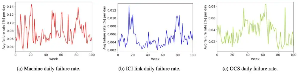
Google's TPU v4 fleet gives per-part rates of the same kind, measured over about two years in production: on average 0.08% of machines, 0.005% of ICI cables and 0.04% of OCSes fail per day (TPU v4 resiliency, NSDI 2024; Figure 10.1).
Google 的 TPU v4 機群給出同類的逐零件故障率,在正式環境量測了約兩年:平均每天有 0.08% 的機器、0.005% 的 ICI 線纜與 0.04% 的 OCS 故障(TPU v4 韌性,NSDI 2024;圖 10.1)。
Cluster MTBF. For a system that stops when any part fails, failure rates add. If part type has rate per unit time and there are of them, the cluster's rate and its mean time between failures (MTBF) are
叢集 MTBF。對一個任何零件故障就會停的系統,故障率相加。若第 種零件每單位時間的故障率是 、數量是 ,叢集的故障率 與平均故障間隔(MTBF) 是
This treats failures as independent and memoryless. It is a first-order model, and the data is not better than first order. A worked example with the numbers above, per month of 30 days, one term per row:
這把故障視為獨立且無記憶。這是一階模型,而資料也不比一階更好。用上面的數字做一個 30 天月份的例子,每列一項:
| Question問題 | Calculation算式 | Result結果 |
|---|---|---|
| GPU-related events per month at Llama's rate (58.7% of 419, scaled from 54 to 30 days)每月 GPU 相關事件,以 Llama 的比率(419 的 58.7%,從 54 天換算到 30 天) | ||
| Cluster rate per month: GPUs + links + ToRs + software bugs at one per day每月叢集故障率 :GPU + 鏈路 + ToR + 每天一次的軟體錯誤 | about 5.9 per day約每天 5.9 次 | |
| Cluster MTBF , with 720 hours in the month叢集 MTBF ,一個月 720 小時 | h小時 | |
| Llama's full count per day (every row of Table 5)Llama 的完整數字,每天(Table 5 的全部項目) | ||
| Llama's MTBFLlama 的 MTBF | h小時 |
The four terms give an MTBF of about 4.1 h (Figure 10.2). Add the host, NIC, maintenance and unknown rows and you reach Llama's full count: 419 in 54 days, 7.8 per day, an MTBF of 3.1 h. Panel 10.3 lets you move every term, and it shows that the GPU term dominates the sum at every scale: doubling the GPUs halves , whatever the network does.
這四項給出約 4.1 小時的 MTBF(圖 10.2)。再加上主機、NIC、維護與不明的項目,你就到達 Llama 的完整數字:54 天 419 次、每天 7.8 次,MTBF 3.1 小時。面板 10.3 讓你移動每一項,並顯示在任何規模下 GPU 項都主導總和:GPU 加倍, 就減半,不管網路做什麼。
Silent data corruption. Silent data corruption (SDC) deserves its own paragraph even at 1.4%. Every other row announces itself: a GPU raises an error, a link goes down, a process dies, a collective times out. An SDC-affected GPU computes a wrong number and reports success. The job keeps training on bad gradients. Detection needs a check that the hardware does not give: a loss that moves in an unexpected way, a disagreement between duplicated computations, or a checksum over exchanged tensors. By the time it is caught, the work since the corruption began may be unusable. The loss is then not half a checkpoint interval but many intervals, and the operator must find the last clean checkpoint, which only exists if old checkpoints are kept.
靜默資料損毀。靜默資料損毀(SDC)即使只占 1.4%,也值得單獨一段。其他每一項都會自我宣告:GPU 拋出錯誤、鏈路斷掉、行程死亡、集體通訊逾時。受 SDC 影響的 GPU 算出錯誤的數字,卻回報成功。任務繼續用壞掉的梯度訓練。偵測需要硬體不提供的檢查:以不尋常方式移動的 loss、重複計算之間的不一致,或交換張量上的校驗和。等到被抓到時,從損毀開始以來的工作可能都不能用。那時損失的不是半個檢查點間隔,而是許多個間隔,而且營運者必須找出最後一個乾淨的檢查點,而那只有在保留舊檢查點時才存在。
10.2Why one failure stops everything為何一次故障就讓一切停下
Synchronous SGD is a barrier. In every step, each rank computes a gradient on its own micro-batch. Then all ranks combine their gradients with an all-reduce, or with a reduce-scatter followed by an all-gather. Then every rank applies the same update. The all-reduce is the barrier. It cannot produce a result without a contribution from every rank, because the sum is not defined until the last term arrives. If one rank is missing, every other rank blocks inside the collective and does no work (Figure 10.3). Nothing in the algorithm distinguishes "rank 4,311 is dead" from "rank 4,311 is slow". After a fixed time the NCCL watchdog declares a timeout and the process group aborts. PyTorch's default timeout for NCCL is 10 minutes. Llama 3's Table 5 lists seven interruptions as "NCCL watchdog timeouts" with unknown cause: a hang that the watchdog ended, and nobody learned why.
同步 SGD 是一道 barrier。每一步,每個 rank 在自己的 micro-batch 上計算梯度。然後所有 rank 用 all-reduce,或用 reduce-scatter 再接 all-gather,把梯度合併。然後每個 rank 套用同一個更新。all-reduce 就是那道 barrier。沒有每個 rank 的貢獻它就無法產生結果,因為在最後一項到達之前總和沒有定義。若一個 rank 缺席,其他每個 rank 都卡在集體通訊裡、什麼事也做不了(圖 10.3)。演算法裡沒有任何東西能區分「rank 4,311 死了」與「rank 4,311 很慢」。經過固定時間後,NCCL watchdog 宣告逾時,行程群組中止。PyTorch 對 NCCL 的預設逾時是 10 分鐘。Llama 3 的 Table 5 把七次中斷列為原因不明的「NCCL watchdog 逾時」:一次被 watchdog 結束的卡死,沒有人知道為什麼。
Effective training time is the share of wall-clock time in which the job makes progress that it keeps. Three terms reduce it on every failure (Figure 10.4). (1) Detection : from the fault to the moment the system knows and acts. With a watchdog alone, is the timeout, 10 minutes. MegaScale's heartbeat cut detection plus diagnosis to under 10 minutes on average, and that figure includes running the diagnostics (MegaScale §4). (2) Restart : tear down the processes, allocate a replacement node, re-initialize the collective groups, load the checkpoint, and warm up. Initialization is a hidden multiplier. Megatron-LM's default initialization took 1,047 s on 2,048 GPUs, because workers registered through a single-threaded blocking store and then ran a global barrier whose cost grew with the square of the worker count. MegaScale brought it under 5 s on 2,048 GPUs and under 30 s on more than 10,000. Every one of their more than 100 restarts paid this cost once; at the old value it would have cost 29 hours in total. (3) Lost work : the computation since the last checkpoint, which must be redone. If failures are not correlated with the checkpoint clock, averages half the interval, . A fourth term applies even with no failure: the checkpoint cost , paid once per interval .
有效訓練時間是任務在其中取得並保留進度的牆上時鐘時間比例。每一次故障有三項會減少它(圖 10.4)。(1) 偵測 :從故障發生到系統得知並採取行動。只靠 watchdog 時, 就是逾時時間,10 分鐘。MegaScale 的心跳把偵測加診斷縮到平均低於 10 分鐘,而這個數字包含執行診斷(MegaScale §4)。(2) 重啟 :關掉行程、分配替換節點、重新初始化集體通訊群組、載入檢查點、暖機。初始化是一個隱藏的乘數。Megatron-LM 的預設初始化在 2,048 顆 GPU 上花 1,047 秒,因為 worker 透過單執行緒的阻塞式儲存註冊,然後執行一個成本隨 worker 數平方成長的全域 barrier。MegaScale 把它壓到 2,048 顆 GPU 低於 5 秒、超過 10,000 顆低於 30 秒。他們超過 100 次重啟的每一次都付了這個成本一次;以舊的數值算,總共會花掉 29 小時。(3) 損失的工作 :自最後一個檢查點以來的計算,必須重做。若故障與檢查點的時鐘不相關, 平均是半個間隔,。第四項即使沒有故障也要付:檢查點成本 ,每個間隔 付一次。
Animation 10.1 plays one interruption, from the fault to the moment the job is back where it was.
動畫 10.1 播放一次中斷:從故障發生,到任務回到原本的進度為止。
The accounting. Put the terms together for one interval of useful work , valid while all terms are small compared with :
算帳。把這些項放在一個有效工作間隔 裡,在所有項都遠小於 時成立:
A worked example from Llama 3: 466 interruptions in 54 days, effective time above 90%. The budget that implies:
用 Llama 3 做一個例子:54 天內 466 次中斷,有效時間高於 90%。這隱含的預算是:
| Question問題 | Calculation算式 | Result結果 |
|---|---|---|
| Most lost time that 90% effective time allows in 54 days54 天內 90% 有效時間所允許的最多損失時間 | min分鐘5.4 days5.4 天 | |
| Average cost per interruption, detection, restart and lost work together每次中斷的平均代價,偵測、重啟與損失的工作合計 | min分鐘 |
So each interruption cost under 16.7 minutes on average. That one inequality tells you two things without any further data: their checkpoints were much closer together than two hours, and their restart was fast. The failure rate sets the budget; the budget sets the engineering. Panel 10.2 adds up for one interruption and compares the sum with this budget.
所以每次中斷平均花費低於 16.7 分鐘。這一個不等式不需要其他資料就告訴你兩件事:他們的檢查點彼此遠比兩小時更近,而且重啟很快。故障率決定預算;預算決定工程。面板 10.2 把一次中斷的 加起來,並與這個預算比較。
10.3Checkpoint arithmetic檢查點的算術
The derivation. This is the Young–Daly result (Young 1974, Daly 2006), and it is short enough to carry in your head. Let the job checkpoint after every of useful work, at a cost . Let failures arrive at random with mean spacing . Per interval, the overhead from checkpointing is of the useful time. Per interval, the chance of a failure is about when is small compared with , and a failure wastes on average. So the overhead fraction is
推導。這是 Young–Daly 的結果(Young 1974、Daly 2006),短到可以記在腦子裡。讓任務每做 的有效工作就存一次檢查點,成本 。讓故障隨機到來,平均間隔 。每個間隔中,檢查點的開銷是有效時間的 。每個間隔中,在 遠小於 時故障的機會約為 ,而一次故障平均浪費 。所以開銷比例是
Differentiate and set to zero: , which gives
微分並設為零:,得到
Substitute back: . Two consequences follow. The minimum overhead depends only on the ratio of checkpoint cost to failure spacing. And halving , or doubling , cuts the minimum overhead by , not by 2. The restart terms add a constant that no choice of can change. Figure 10.5 draws the two terms and their sum.
代回去:。兩個結論隨之而來。最小開銷只取決於檢查點成本與故障間隔的比值 。而 減半或 加倍,最小開銷只減少 倍,不是 2 倍。重啟項 加上一個常數 ,任何 的選擇都改變不了它。圖 10.5 畫出這兩項與它們的總和。
Animation 10.2 sweeps the checkpoint interval and shows where one mean time between failures goes.
動畫 10.2 掃過不同的檢查點間隔,顯示一個平均故障間隔的時間花到哪裡去。
Worked example. Take s and compare two checkpoint costs: s, the pause of a two-stage copy to host memory, and s, a direct write of a few hundred terabytes to a distributed file system. Detection plus restart is min. The arithmetic, one question per row:
算例。取 秒,比較兩種檢查點成本: 秒,兩階段複製到主機記憶體的暫停;以及 秒,直接把幾百 TB 寫進分散式檔案系統。偵測加重啟 分鐘。逐列計算如下:
| Question問題 | Calculation算式 | Result結果 |
|---|---|---|
| Best interval at s 秒時的最佳間隔 | sabout 15.5 min約 15.5 分鐘 | |
| Minimum overhead at s 秒時的最小開銷 | ||
| Restart term 重啟項 | ||
| Total overhead at s 秒時的總開銷 | effective time ≈ 89%有效時間 ≈ 89% | |
| Best interval at s 秒時的最佳間隔 | sabout 49 min約 49 分鐘 | |
| Minimum overhead at s 秒時的最小開銷 | ||
| What a tenfold cheaper checkpoint does to and 便宜十倍的檢查點對 與 的影響 | lower overhead, shorter interval開銷更低、間隔更短 |
With the cheap checkpoint the job checkpoints every 15.5 minutes and keeps about 89% of its time; the expensive one stretches the best interval to 49 minutes and the minimum overhead to 20.4%. A tenfold cheaper checkpoint cuts the minimum overhead by about 3.2× and allows a 3.2× shorter interval. The checkpoint cost, not the failure rate, is the lever that an engineer controls.
便宜的檢查點讓任務每 15.5 分鐘存一次、保留約 89% 的時間;昂貴的則把最佳間隔拉長到 49 分鐘、最小開銷升到 20.4%。便宜十倍的檢查點把最小開銷減少約 3.2 倍,並允許短 3.2 倍的間隔。工程師能控制的槓桿是檢查點成本,不是故障率。
What HPN observed. HPN §2.2 reports that jobs checkpointed every 2 to 4 hours. With h and h, a failure loses h on average, which is 37% of the time between failures, before counting restart. That is why HPN's authors describe one ToR failure as destroying hours of GPU time, and why they treat reliability as a topology problem (Section 10.5 below). Long intervals come from a high : a full checkpoint of a 175B-parameter model written straight to a distributed file system takes minutes and hammers the storage with thousands of simultaneous writers. The formula says the fix is to make small, and the two systems below did exactly that.
HPN 觀察到的。HPN §2.2 報告任務每 2 到 4 小時存一次檢查點。用 小時與 小時,一次故障平均損失 小時,是故障間隔時間的 37%,還沒算重啟。這就是 HPN 作者把一次 ToR 故障描述成毀掉數小時 GPU 時間的原因,也是他們把可靠性當成拓樸問題處理的原因(下面 第 10.5 節)。長間隔來自高 :把 1,750 億參數模型的完整檢查點直接寫進分散式檔案系統要花數分鐘,而且數千個同時寫入者會把儲存打垮。公式說解法是把 變小,而下面兩個系統正是這麼做。
Two-stage checkpoints. MegaScale's two-stage checkpoint separates the pause from the write. Stage one copies each GPU's state to pinned host memory over PCIe; the job pauses for seconds. Stage two writes from host memory to HDFS in the background while training continues. The in the Young–Daly formula is the pause, not the write. A size check: Llama 3's checkpoints are 1 MB to 4 GB per GPU depending on sharding. Take the largest:
兩階段檢查點。MegaScale 的兩階段檢查點把暫停與寫入分開。第一階段透過 PCIe 把每顆 GPU 的狀態複製到釘住的主機記憶體;任務暫停數秒。第二階段在訓練繼續的同時,在背景把主機記憶體寫到 HDFS。Young–Daly 公式裡的 是暫停,不是寫入。檢查一下大小:Llama 3 的檢查點依分片方式每顆 GPU 從 1 MB 到 4 GB。取最大的:
| Question問題 | Calculation算式 | Result結果 |
|---|---|---|
| Copy 4 GB to host memory over a PCIe 5.0 x16 slot at about 64 GB/s透過約 64 GB/s 的 PCIe 5.0 x16 插槽把 4 GB 複製到主機記憶體 | swell under a second遠不到一秒 | |
| One checkpoint at 4 GB per GPU on 16,384 GPUs16,384 顆 GPU、每顆 4 GB 的一個檢查點 | TB | |
| Drain it at Tectonic's 7 TB/s peak (Llama 3 §3.3.1)以 Tectonic 的 7 TB/s 峰值排空(Llama 3 §3.3.1) | s | |
| Drain it at Tectonic's 2 TB/s sustained rate以 Tectonic 的 2 TB/s 持續速率排空 | s |
The copy to host memory takes well under a second, so the seconds that MegaScale reports are software overhead, not bandwidth. The write is the storage system's problem: 65.5 TB per checkpoint, 9 s at Tectonic's peak and 33 s at its sustained rate. This is the bursty write that Llama's authors call a major challenge, and it is why the front-end network and the storage are sized for peaks, not averages (see Chapter 9). Recovery reads are made cheap in the same spirit: one reader per data-parallel group fetches the shard from HDFS and broadcasts it to the rest over the back-end network, so the file system serves tens of readers instead of thousands.
複製到主機記憶體遠不到一秒,所以 MegaScale 報告的「數秒」是軟體開銷,不是頻寬。寫入是儲存系統的問題:每個檢查點 65.5 TB,以 Tectonic 的峰值要 9 秒、持續速率要 33 秒。這就是 Llama 作者稱為主要挑戰的突發寫入,也是前端網路與儲存依峰值而非平均值定尺寸的原因(見第 9 章)。恢復時的讀取也以同樣精神變便宜:每個資料平行群組一個讀取者從 HDFS 抓取分片,再透過後端網路廣播給其他成員,所以檔案系統只服務數十個讀取者而非數千個。
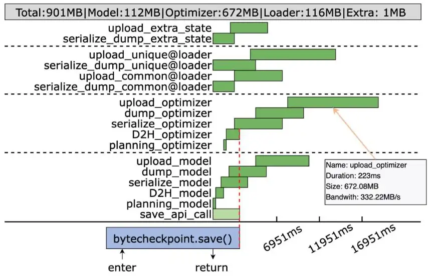
ByteDance's later ByteCheckpoint system shows the same split in a measured trace of one save (ByteCheckpoint, NSDI 2025; Figure 10.6): the training loop waits only for planning and the device-to-host copies.
字節跳動後來的 ByteCheckpoint 系統,在一次儲存的實測紀錄中顯示同樣的分割(ByteCheckpoint,NSDI 2025;圖 10.6):訓練迴圈只等待規劃與裝置到主機的複製。
At Llama's rate the Young–Daly minimum, , is about 7% for s. To stay above 90% in total, the constant term must be under 3%, so detection plus restart must average under about 5 minutes. Use Panel 10.3 to find the largest that still gives 90% at , then raise to 120 s and see how much faster the restart must become to compensate. This is why MegaScale's initialization fix, 1,047 s to under 5 s, belongs in a reliability section.
在 Llama 的故障率下,Young–Daly 的最小值 在 秒時約為 7%。要讓總和保持在 90% 以上,常數項 必須低於 3%,所以偵測加重啟平均必須低於約 5 分鐘。用面板 10.3 找出在 下仍能給 90% 的最大 ,然後把 提高到 120 秒,看重啟必須快多少才能補償。這就是 MegaScale 把初始化從 1,047 秒壓到 5 秒以下的修正為何屬於可靠性章節的原因。
10.4Automated recovery loops自動化恢復迴圈
Mechanism. MegaScale turns recovery into a workflow with no operator in it (MegaScale §4). A driver process requests resources from Kubernetes and starts one executor per node, which launches the training processes. Each executor runs a daemon that sends a heartbeat to the driver. The heartbeat carries the node's IP address and pod name, hardware information, the training process status, its stdout and stderr logs, and the RDMA traffic counters of its NICs. The counters are the key signal. Training traffic is periodic and regular: every step runs the same collectives in the same order (in a mixture-of-experts model the all-to-all destinations change from step to step, but the steps still repeat), so a sudden drop raises an alert and traffic that stops entirely triggers recovery automatically, before any process has reported an error. When the driver sees an anomaly, or no heartbeat at all, it suspends the job and runs a battery of diagnostics on the suspect nodes: an intra-host loopback test from every NIC to host memory and to the GPUs, a NIC-to-NIC connectivity and bandwidth test, an NCCL all-to-all within the node, and an NCCL all-reduce with the neighboring nodes under the same ToR. Each test isolates one layer (Figure 10.7), so a result of "loopback passes, NIC-to-NIC fails" points at the link rather than the host. Nodes that fail are evicted and replaced from a standby pool, and the job restarts from the last checkpoint.
機制。MegaScale 把恢復變成一個沒有營運人員在其中的工作流程(MegaScale §4)。一個 driver 行程向 Kubernetes 申請資源,並在每個節點啟動一個 executor,由它啟動訓練行程。每個 executor 跑一個 daemon,向 driver 送心跳。心跳帶著節點的 IP 位址與 pod 名稱、硬體資訊、訓練行程狀態、它的 stdout 與 stderr 日誌,以及其 NIC 的 RDMA 流量計數器。計數器是關鍵訊號。訓練流量是週期性且規律的:每一步都以相同順序執行相同的集體操作(混合專家模型的 all-to-all 目的地每步都不同,但步驟本身仍然重複),所以突然下降就發出警報,完全停止就自動觸發恢復,在任何行程回報錯誤之前。當 driver 看到異常,或完全收不到心跳,它暫停任務並對可疑節點執行一組診斷:每張 NIC 到主機記憶體與 GPU 的主機內迴路測試、NIC 對 NIC 的連通性與頻寬測試、節點內的 NCCL all-to-all,以及與同一 ToR 下鄰近節點的 NCCL all-reduce。每個測試隔離一層(圖 10.7),所以「迴路通過、NIC 對 NIC 失敗」的結果指向鏈路而不是主機。失敗的節點被逐出並從備用池替換,任務從最後的檢查點重啟。
Why the loop and not a person. A person takes tens of minutes to notice a hang, read logs across thousands of nodes and decide which node to drain. At 7.8 interruptions per day, that alone would consume the 10% budget from Section 10.2. The loop also removes the most expensive failure mode: the one nobody notices. A job that hangs at 03:00 and is found at 09:00 has lost six hours of 16,000 GPUs, about 100,000 GPU-hours, from one event. MegaScale's numbers: in a production run of several weeks on more than 10,000 GPUs, training restarted more than 100 times; more than 90% of the software and hardware faults were handled with no human involvement; detection plus diagnosis took under 10 minutes on average; and the job caught up to its pre-failure progress within 15 minutes of the last checkpoint, keeping effective training time above 90%. Llama 3 reports the same shape at 16K GPUs: 466 interruptions in 54 days, 47 of them planned (firmware and kernel upgrades, configuration changes, dataset updates), and only three that needed significant manual intervention.
為什麼要迴圈而不是人。一個人要花數十分鐘才會注意到卡死、讀遍數千個節點的日誌、決定要排空哪個節點。在每天 7.8 次中斷下,光這一項就會吃掉 第 10.2 節 的 10% 預算。這個迴圈也移除了最昂貴的故障模式:沒有人注意到的那種。一個在 03:00 卡死、09:00 才被發現的任務,一次事件就損失了 16,000 顆 GPU 的六小時,約 100,000 GPU-小時。MegaScale 的數字:在超過 10,000 顆 GPU 上數週的生產運行中,訓練重啟超過 100 次;超過 90% 的軟硬體故障在沒有人介入下處理完畢;偵測加診斷平均低於 10 分鐘;任務在最後檢查點之後 15 分鐘內追回故障前的進度,有效訓練時間維持在 90% 以上。Llama 3 在 16K GPU 上報告同樣的形態:54 天內 466 次中斷,其中 47 次是預期內的(韌體與核心升級、設定變更、資料集更新),只有三次需要顯著的人工介入。
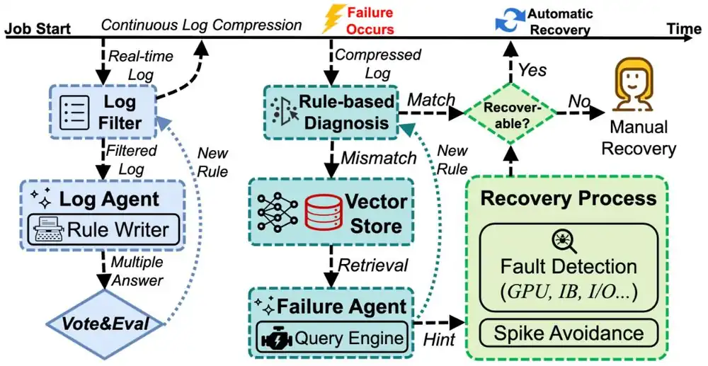
Shanghai AI Laboratory's Acme datacenter splits recovery the same way (Acme, NSDI 2024; Figure 10.8): automatic recovery when the diagnosis says the fault is recoverable, a person when it is not. Its authors estimate, roughly, that the diagnosis system cut manual intervention by about 90%.
上海人工智慧實驗室的 Acme 資料中心用同樣的方式分割恢復(Acme,NSDI 2024;圖 10.8):診斷判定故障可恢復時自動恢復,否則交給人。作者粗估這套診斷系統讓人工介入減少約 90%。
Animation 10.3 plays MegaScale's loop for a fault that it handles and for one that escapes it.
動畫 10.3 播放 MegaScale 的迴圈:一次它能處理的故障,與一次逃出它的故障。
The arithmetic with those numbers. Take MegaScale first: "more than 100 restarts in several weeks", reading several as three. Then Llama 3: the 7,776 lost minutes allowed by 90% over 54 days, divided by 466, gave 16.7 minutes per interruption in Section 10.2, and the three manual interventions are the risk in that budget; suppose each took four hours. One question per row:
用這些數字算一算。先看 MegaScale:「數週內超過 100 次重啟」,把「數週」當成三週。再看 Llama 3:90% 在 54 天內允許的 7,776 分鐘損失除以 466,在 第 10.2 節 得到每次中斷 16.7 分鐘,而三次人工介入是這個預算裡的風險;假設每次花四小時。逐列計算如下:
| Question問題 | Calculation算式 | Result結果 |
|---|---|---|
| MegaScale: spacing of 100 restarts in three weeksMegaScale:三週 100 次重啟的間隔 | h小時 | |
| Wall-clock loss per restart: diagnosis under 10 min, catch-up within 15 min每次重啟的牆上時鐘損失:診斷低於 10 分鐘、15 分鐘內追回 | min分鐘 | |
| Share of time lost損失的時間比例 | effective time ≈ 92%有效時間 ≈ 92% | |
| Llama 3: three manual interventions at four hours eachLlama 3:三次人工介入、每次四小時 | min分鐘 | |
| Their share of the 7,776-minute budget占 7,776 分鐘預算的比例 | ||
| Their share of the 466 interruptions占 466 次中斷的比例 |
MegaScale's effective time of about 92% is consistent with the paper's "above 90%". For Llama 3, 0.6% of the events would consume 9% of the whole budget. That is the general rule of recovery loops: the automated 90% sets the average, and the manual 10% sets the variance. The design goal is not a faster average but fewer events that escape the loop. Panel 10.4 lets you trade automated recovery time against the events that escape.
MegaScale 約 92% 的有效時間與論文的「高於 90%」一致。對 Llama 3 而言,只占 0.6% 的事件就會吃掉整個預算的 9%。這是恢復迴圈的通則:自動化的 90% 決定平均值,人工的 10% 決定變異。設計目標不是更快的平均,而是更少逃出迴圈的事件。面板 10.4 讓你在自動恢復時間與逃出迴圈的事件之間取捨。
10.5Designing so that failures hurt less讓故障傷害更小的設計
Section 10.3 showed that the cost of a failure is , , and , and Section 10.4 showed how to shrink and . The remaining lever is to stop a fault from being a failure at all: to let the job continue, slower, while the part is repaired. Six published mechanisms do this, each with a number attached.
第 10.3 節 顯示一次故障的成本是 、、 與 ,第 10.4 節 顯示如何縮小 與 。剩下的槓桿是讓一個缺陷根本不成為故障:讓任務在零件修復期間以較慢的速度繼續。有六個已發表的機制做到這件事,每個都附帶一個數字。
Dual-ToR without stacking (HPN §4). Each NIC has two 200G ports wired to two rack switches that share nothing: no inter-switch link, no shared state. The host bonds the two ports under one IP and one MAC and sends its address announcements (ARP) to both switches, which turn them into routes for the network above; the host runs no routing protocol itself. When a link or a ToR fails, the host stops using that port (Section 6.5). In HPN's experiment on 256 GPUs training LLaMa-7B, failing a single NIC–ToR link cost 6.25% of training throughput, which is one of the sixteen 200G ports on a host, and throughput returned to normal when the link was repaired. In the single-ToR baseline the job halted, and if the repair took more than two minutes it could not recover at all. A link flap that stalled single-ToR training for more than nine seconds was negligible under dual-ToR. The usual stacked alternative (vPC, M-LAG) is rejected with a fleet number: more than 40% of critical failures in Alibaba's traditional data centers came from the stacked design, because a switch whose data plane dies while its control plane lives makes its healthy peer shut down too.
不堆疊的 dual-ToR(HPN §4)。每張 NIC 有兩個 200G 埠,接到兩台什麼都不共享的機櫃交換器:沒有交換器之間的鏈路、沒有共享狀態。主機把兩個埠綁在一個 IP 與一個 MAC 之下,把位址宣告(ARP)送給兩台交換器,由交換器把它轉成給上層網路的路由;主機本身不跑路由協定。當鏈路或 ToR 故障,主機就不再使用那個埠(第 6.5 節)。在 HPN 於 256 顆 GPU 上訓練 LLaMa-7B 的實驗中,弄斷一條 NIC–ToR 鏈路損失 6.25% 的訓練吞吐,即主機十六個 200G 埠之一,鏈路修復時吞吐就恢復正常。在單 ToR 基線中任務停擺,而若修復超過兩分鐘就完全無法恢復。一次讓單 ToR 訓練停擺超過九秒的鏈路抖動,在 dual-ToR 下可忽略。常見的堆疊式替代方案(vPC、M-LAG)被一個機群數字否決:阿里傳統資料中心超過 40% 的重大故障來自堆疊設計,因為一台資料平面死掉但控制平面還活著的交換器,會讓健康的同儕也關機。
Backup hosts per segment (HPN §5.1). Each HPN ToR reserves 8 of its 136 host-facing ports as backups, so a segment of 1,024 active GPUs carries 64 spare GPUs, 6.25% again. When a host fails, the job restarts on a spare in the same segment, with the same single-hop reach to its peers, instead of waiting for a repair or being re-placed across the pod. The spares also change the decision after a link failure. Under dual-ToR the degraded host costs 6.25% of throughput for the whole repair time . Swapping the host to a spare costs one restart from the checkpoint instead: . The swap is worth it when , that is, when
每個 segment 的備用主機(HPN §5.1)。每台 HPN ToR 把 136 個面向主機的埠中保留 8 個作為備援,所以一個有 1,024 顆使用中 GPU 的 segment 帶著 64 顆備用 GPU,又是 6.25%。主機故障時,任務在同一 segment 的備用機上重啟,與同儕保持同樣的單跳可達,而不必等修復或被重新配置到 pod 的其他地方。備用機也改變鏈路故障後的決策。在 dual-ToR 下,降級的主機在整個修復時間 內損失 6.25% 的吞吐。把主機換到備用機則只花一次從檢查點重啟的成本:。當 時換機划得來,即
With a 15-minute interval and a 5-minute restart, that is a repair longer than about 3.3 hours; with HPN's 2-hour interval it is about 17 hours. Panel 10.5 computes this break-even for you.
用 15 分鐘的間隔與 5 分鐘的重啟,那是超過約 3.3 小時的修復;用 HPN 的 2 小時間隔則約 17 小時。面板 10.5 會替你算這個損益平衡點。
Uplink headroom (Meta RoCE §6). Meta's rack switches moved from 1:1 to 1:2 uplink bandwidth during tuning, then settled at 1:1.125: enough headroom to tolerate two failed uplinks without slowing a job, at far lower cost than 1:2. The arithmetic: with uplinks, two failures leave of the uplink capacity. The rack stays non-blocking when , which requires . The rule generalizes: to survive failed uplinks out of at full rate, you need a ratio of . Fewer, fatter uplinks need more headroom per link lost. The same paper lists the alarms that make a degraded link visible before it becomes a stall: out-of-sequence packet counters on the NICs (a sign of loss or reordering), link flaps, local ACK timeouts, a PFC watchdog that fires when a port stays paused for 200 ms, buffer alarms when a cluster switch buffer passes 80%, and periodic reachability pings between all hosts. Two incidents show why: a switch software upgrade raised port-to-port latency and silently slowed training until the monitoring caught it, and an outdated assumption about SRAM buffer carving caused tail drops whenever more than half the buffer was in use (Meta RoCE).
上行餘裕(Meta RoCE §6)。Meta 的機櫃交換器在調校期間從 1:1 的上行頻寬改到 1:2,然後定在 1:1.125:足以容忍兩條上行故障而不拖慢任務,成本又遠低於 1:2。算術如下:有 條上行時,兩條故障留下 的上行容量。當 時機櫃維持非阻塞,這需要 。這個規則可以推廣:要在 條中失去 條上行後仍全速運行,需要 的比例。更少、更粗的上行每失去一條就需要更多餘裕。同一篇論文列出讓降級鏈路在變成停擺之前就被看見的警報:NIC 上的亂序封包計數器(丟包或重排序的徵兆)、鏈路抖動、本地 ACK 逾時、一個埠持續暫停 200 ms 就觸發的 PFC watchdog、叢集交換器緩衝超過 80% 的緩衝警報,以及所有主機之間週期性的可達性 ping。兩起事故說明原因:一次交換器軟體升級提高了埠對埠延遲並悄悄拖慢訓練直到監控抓到;一個關於 SRAM 緩衝切割的過時假設讓緩衝使用超過一半就出現尾端丟包(Meta RoCE)。
Rerouting the torus (TPU v4, ISCA 2023, §2.3). Google's argument for optical circuit switches leads with availability. Figure 10.4 of that paper plots goodput, the useful work delivered, against host availability from 99.0% to 99.9%. Without OCSes, a fixed torus delivers reasonable goodput only at 99.9% host availability; with OCSes, the scheduler picks other cubes and rewires the torus around the failure, and goodput is acceptable at 99.0–99.5% (TPU v4). The arithmetic behind the curve is a power. A fixed slice of hosts is usable only when all are up, with probability . For hosts:
重新接線的環面(TPU v4,ISCA 2023,§2.3)。Google 支持光路交換器的論證以可用性開頭。該論文的 Figure 4 畫出 goodput(交付的有用工作)隨主機可用性從 99.0% 到 99.9% 的變化。沒有 OCS 時,固定環面只在 99.9% 的主機可用性下有合理的 goodput;有 OCS 時,排程器挑其他 cube 並把環面繞過故障重新接線,goodput 在 99.0–99.5% 下仍可接受(TPU v4)。曲線背後的算術是一個次方。 台主機的固定切片只有在全部 台都正常時可用,機率為 。以 台主機計:
| Question問題 | Calculation算式 | Result結果 |
|---|---|---|
| All 256 hosts up at 99.9% host availability主機可用性 99.9% 時 256 台全部正常 | ||
| All 256 hosts up at 99.5%99.5% 時 256 台全部正常 | ||
| All 256 hosts up at 99.0%99.0% 時 256 台全部正常 |
At 99.0% availability a fixed 256-host slice is whole only 8% of the time. A reconfigurable slice needs only 256 working hosts out of a larger pool, which is nearly always true. Spare capacity is the limit for very large slices: a slice of one quarter of the machine reaches 75% goodput at those availabilities.
在 99.0% 的可用性下,一個固定的 256 主機切片只有 8% 的時間是完整的。可重構的切片只需要在更大的池子裡找出 256 台正常主機,這幾乎永遠成立。備用容量是極大切片的限制:占整台機器四分之一的切片在那些可用性下達到 75% 的 goodput。
Those curves are the design argument. The measured counterpart comes from Google's later operations paper (TPU v4 resiliency, NSDI 2024): job availability against job size in deployed pods (the figure in Section 6.9). Its headline of 99.98% availability has no definition or method in the paper, so this chapter does not use it as a measured number.
那些曲線是設計上的論證。量測上的對照來自 Google 後來的營運論文(TPU v4 韌性,NSDI 2024):已部署 pod 中任務可用度對任務規模的關係(第 6.9 節的圖)。它標題上的 99.98% 可用度在論文中沒有定義也沒有方法,所以本章不把它當成量測數字。
Riding through flaps (MegaScale §3.6 and §6.3). A flap drops the packets in flight and then restores the link within seconds. The danger is not the lost packets but the timers around them. In MegaScale's case study, interfaces went down for several seconds, the default NCCL timeout expired before the NIC recovered, and the job died. Setting a larger timeout explicitly let the job ride through. ByteDance also tuned NCCL's retransmit timer and retry count, and enabled the NIC's adaptive retransmission so that retries happen at shorter intervals. The root cause was poor signal quality across the NIC, the active optical cable and the switch port, fixed with tighter quality control on cabling. Under HPN's dual-ToR the same event is invisible, because the host simply uses the other port for those seconds.
撐過抖動(MegaScale §3.6 與 §6.3)。一次抖動丟掉在途的封包,然後在數秒內恢復鏈路。危險的不是丟掉的封包,而是圍繞它們的計時器。在 MegaScale 的案例中,介面斷線數秒,預設的 NCCL 逾時在 NIC 恢復前到期,任務就死了。明確設定較大的逾時讓任務得以撐過。字節跳動也調校了 NCCL 的重傳計時器與重試次數,並啟用 NIC 的自適應重傳,讓重試以更短的間隔進行。根本原因是 NIC、主動光纜與交換器埠之間的訊號品質不佳,以更嚴格的線纜品質管控修正。在 HPN 的 dual-ToR 下同一事件是看不見的,因為主機在那幾秒就是改用另一個埠。
The asymmetric link (HPN §10). A production incident at Alibaba came from a link whose optical signal was bad in the NIC-to-ToR direction but fine in the other. The ToR detected the fault and tried to tell the NIC through Link Fault Signaling, but a NIC firmware bug ignored the message. The NIC kept sending on a link it believed healthy, and packets were lost at scale. No testbed produces this fault, and no watchdog on the switch can fix a host that will not listen. Dual-ToR turned it from a crash into a slowdown, which is the whole point of the design: it does not need to know why a port is bad to stop using it.
非對稱鏈路(HPN §10)。阿里的一次生產事故來自一條在 NIC 到 ToR 方向光訊號不良、另一方向卻正常的鏈路。ToR 偵測到故障並嘗試透過 Link Fault Signaling 通知 NIC,但 NIC 韌體的錯誤忽略了訊息。NIC 持續在它以為健康的鏈路上發送,大量封包遺失。沒有任何測試環境會產生這種故障,交換器上的任何 watchdog 也修不了一台不聽話的主機。Dual-ToR 讓它從崩潰變成減速,而這正是這個設計的重點:它不需要知道一個埠為何壞掉,就能停止使用它。
Dual-ToR doubles the number of links, so it doubles the link events. Why does it still win? Use Panel 10.5 with HPN's 2-hour interval and compare the lost GPU-hours of single-ToR and dual-ToR. Then shorten the interval to 15 minutes, as Panel 10.3 recommends, and watch the gap shrink: the cheaper a halt becomes, the less a design that avoids halts is worth. At what interval and repair time do the two designs tie?
Dual-ToR 讓鏈路數加倍,所以鏈路事件也加倍。為什麼它還是贏?用面板 10.5 設 HPN 的 2 小時間隔,比較單 ToR 與 dual-ToR 損失的 GPU-小時。然後把間隔縮到面板 10.3 建議的 15 分鐘,看差距縮小:停擺越便宜,一個避免停擺的設計就越不值錢。在什麼間隔與修復時間下兩種設計打平?
10.6Stragglers: the cost of the slowest rank落後者:最慢的 rank 的代價
Mechanism. The barrier of Section 10.2 has a second consequence. The step time of a synchronous job is not the average rank's time but the maximum over all ranks, because the collective completes when the last contribution arrives. A host that is 10% slower makes the whole job 10% slower, however many thousands of healthy hosts there are (Figure 10.9). A straggler is a rank that is persistently slower than its peers; jitter is the random variation that every rank shows from step to step. Both are paid through the same maximum, and the network sees both as the same thing: ranks that finish their compute late issue their collectives late, and the other ranks wait in the collective, so the wait is recorded as communication time even when the cause is a slow GPU.
機制。第 10.2 節 的 barrier 有第二個後果。同步任務的步時間不是平均 rank 的時間,而是所有 rank 之中的最大值,因為集體通訊在最後一份貢獻到達時才完成。一台慢 10% 的主機讓整個任務慢 10%,不管有幾千台健康的主機(圖 10.9)。Straggler 是持續比同儕慢的 rank;jitter 則是每個 rank 每一步都會出現的隨機變化。兩者都透過同一個最大值付出代價,而網路把兩者看成同一件事:計算較晚完成的 rank 較晚發出集體通訊,其他 rank 在集體通訊裡等待,所以即使原因是慢的 GPU,等待仍被記成通訊時間。
MegaScale's numbers. A CUDA event monitor timed critical code segments on every rank with CUDA events rather than host timers, so it did not force the GPU to synchronize and could stay on in production. Its heat map of per-rank step times showed that about 0.5% of machines were substantially slower than the rest, and because every collective waits for its slowest member, that 0.5% set the pace for everyone. Excluding those machines made peak MFU consistent from run to run (MegaScale §5). In the case study of §6.3, some hosts took about 10% longer on identical forward computations; isolating and removing them gained about 0.7 MFU points. Check the arithmetic, assuming the slow hosts were 10% slower on the forward computation only:
MegaScale 的數字。一個 CUDA 事件監控器用 CUDA 事件而非主機計時器為每個 rank 的關鍵程式段計時,所以它不強迫 GPU 同步,可以在生產環境常開。它的逐 rank 步時間熱圖顯示約 0.5% 的機器明顯比其他慢,而因為每個集體通訊都等最慢的成員,那 0.5% 決定了所有人的節奏。排除那些機器後峰值 MFU 在各次運行間變得一致(MegaScale §5)。在 §6.3 的案例中,某些主機在相同的正向計算上多花約 10%;隔離並移除它們拿回約 0.7 個 MFU 百分點。驗算一下,假設慢的主機只在正向計算上慢 10%:
| Question問題 | Calculation算式 | Result結果 |
|---|---|---|
| Throughput change from 0.7 MFU points at 55.2% MFU在 55.2% MFU 下 0.7 點的吞吐變化 | the step got about 1.3% shorter步時間縮短約 1.3% | |
| Forward computation's share of the step, if it ran 10% slower正向計算占步時間的比例(若它慢了 10%) |
So the forward computation was about 13% of the step. A straggler costs the whole job its slowdown times the share of the step it slows. The paper's second case is pure jitter: MFU declined slowly over a long run because some ranks launched their gradient reduce-scatter later than others; the cause was irregular Python garbage collection and a few PyTorch operations on the critical path, and removing them stopped the decline.
所以正向計算約占步時間的 13%。一個 straggler 讓整個任務付出的成本是它的減速乘上它拖慢的那部分步時間的比例。論文的第二個案例是純粹的 jitter:長時間運行中 MFU 緩慢下滑,因為某些 rank 比其他 rank 更晚發出梯度 reduce-scatter;原因是不規律的 Python 垃圾回收與關鍵路徑上的幾個 PyTorch 操作,移除後下滑就停止。
Animation 10.4 plays four steps with a 10% straggler, its detection and its replacement.
動畫 10.4 播放四個步驟:一個慢 10% 的 straggler、它被偵測出來,以及被替換。
Llama 3's observations. Meta notes that a single straggler can slow thousands of GPUs, and built tooling that ranks suspect communications from chosen process groups and lets engineers inspect the top few. The PyTorch NCCL flight recorder, a ring buffer of recent collective calls with their state, supported this; so did the ability to change configuration online, without a restart. Llama also reports a diurnal effect: throughput varied by 1–2% over each day in step with mid-day temperature, because hotter GPUs lower their clock through dynamic voltage and frequency scaling. That is a straggler made by the weather: the hottest rack in the building sets the step time for the whole job, twice a day. MegaScale's third tool, a 3-D parallel visualizer, draws the tensor, pipeline and data-parallel groups and the data flow between ranks; when a collective times out, every healthy rank logs the operation it was waiting on while the faulty rank has hung and logs nothing, and the silent rank is the one to drain.
Llama 3 的觀察。Meta 指出單一 straggler 就能拖慢數千顆 GPU,並建了工具,對選定行程群組的可疑通訊排序,讓工程師檢查前幾名。PyTorch 的 NCCL flight recorder(保留近期集體呼叫及其狀態的環形緩衝)支持了這件事;不必重啟就能線上修改設定的能力也是。Llama 也報告一個日夜效應:吞吐每天隨正午溫度有 1–2% 的變化,因為較熱的 GPU 透過動態電壓與頻率調節降低時脈。那是天氣製造出來的 straggler:建築裡最熱的機櫃每天兩次決定整個任務的步時間。MegaScale 的第三個工具,3-D 平行可視化工具,畫出張量、管線與資料平行群組以及 rank 之間的資料流;當集體通訊逾時,每個健康的 rank 記錄它正在等待的操作,而故障的 rank 已經卡住、什麼都沒記,那個沉默的 rank 就是該排空的那個。
The order-statistics view. Even with no chronic straggler, jitter, the small random variation of each rank's step time, costs more as the job grows. Suppose each rank's step time varies independently with standard deviation around the same mean. The step time is the maximum of such values. For Gaussian jitter and large , the expected maximum grows like
順序統計量的觀點。即使沒有長期的 straggler,jitter(每個 rank 步時間小而隨機的變化)的成本也隨任務成長而增加。假設每個 rank 的步時間繞著同一個平均值獨立變動,標準差為 。步時間就是 個這種值的最大值。對高斯 jitter,期望最大值在 很大時隨下式成長:
The exact expectation, computed from the distribution of the maximum, compares with the asymptotic formula like this:
由最大值的分布算出的精確期望值,與漸近公式的比較如下:
| Exact 精確 | Formula 公式 | Formula too high by公式高估 | |
|---|---|---|---|
| 64 | 23% | ||
| 1,024 | 15% | ||
| 16,384 | 11% | ||
| 131,072 | 9% |
The formula is an upper estimate that tightens as grows (Figure 10.10). The growth is slow, which is the good news, but it never stops, and it multiplies whatever the hardware and software provide. With at 16K ranks, every step is about 4% longer than a typical rank needs, with no part broken and nothing to repair. The lever is : pin the garbage collector, keep the critical path free of host-side work, cool the racks evenly, and keep the network's tail latency low, because the network's own jitter adds to . Panel 10.6 runs this experiment with a chronic-straggler population added, and reproduces the 0.7 MFU points of MegaScale.
這個公式是偏高的估計, 越大越準(圖 10.10)。成長很慢,這是好消息,但它永不停止,而且它放大硬體與軟體提供的任何 。在 16K 個 rank 下 ,每一步比一般 rank 所需長約 4%,沒有任何零件壞掉、沒有任何東西要修。槓桿是 :釘住垃圾回收器、讓關鍵路徑不含主機端工作、讓機櫃散熱均勻、讓網路的尾端延遲維持低,因為網路自己的 jitter 會加進 。面板 10.6 加上一群長期 straggler 來跑這個實驗,並重現 MegaScale 的 0.7 個 MFU 百分點。
Set the chronic stragglers to zero and to 0.5%. Read the mean inflation at and at . The ratio of the two is the price of scale with no broken parts. Now set to 0.25%: the inflation halves at both sizes. To get the same halving by shrinking the job, you would have to go from 65,536 ranks to about 40, because the maximum grows only logarithmically. That is why MegaScale spends a section on garbage collection and Llama on a flight recorder: is the lever, not .
把長期 straggler 設為零、 設為 0.5%。讀出 與 時的平均膨脹。兩者的比值就是在沒有零件壞掉下規模的代價。現在把 設為 0.25%:兩種規模的膨脹都減半。要靠縮小任務得到同樣的減半,你得從 65,536 個 rank 縮到約 40 個,因為最大值只以對數成長。這就是 MegaScale 花一節談垃圾回收、Llama 談 flight recorder 的原因:槓桿是 ,不是 。
A synchronous job is a series system: it runs only while every part works, so failure rates add. Llama 3's 16,384 GPUs saw 419 unexpected interruptions in 54 days, one every three hours, mostly GPUs and their memory; the network was about a tenth. One dead rank stops all the others, because the collective cannot finish without it; each interruption costs detection, restart and the work since the last checkpoint. The Young–Daly rule gives the best checkpoint interval, the square root of 2 × checkpoint cost × MTBF; cheap two-stage checkpoints allow short intervals. Automated loops detect, diagnose and restart without a person; wiring (dual-ToR, backup hosts, spare uplinks, optical switches) turns failures into slowdowns. Even without failures, a step lasts as long as its slowest rank, and the expected slowest of N grows like σ√(2 ln N).
同步任務是一個串聯系統:只有每個零件都正常時才能運行,所以故障率相加。Llama 3 的 16,384 顆 GPU 在 54 天內遇到 419 次非預期中斷,約每三小時一次,大多來自 GPU 與其記憶體;網路約占十分之一。一個死掉的 rank 會讓其他所有 rank 停下,因為少了它集體操作就無法完成;每次中斷都要付出偵測、重啟,以及上一個檢查點之後的工作。Young–Daly 法則給出最佳檢查點間隔:2 × 檢查點成本 × MTBF 的平方根;便宜的兩階段檢查點容許很短的間隔。自動化迴圈不需人工就能偵測、診斷與重啟;接線(雙 ToR、備用主機、多餘的上行、光路交換器)把故障變成減速。即使沒有故障,一步的長度仍由最慢的 rank 決定,而 N 個 rank 中最慢者的期望值隨 σ√(2 ln N) 成長。
Chapter 11 looks at clusters shared by many jobs: where each job is placed, what that does to the network, and how jobs disturb one another.
第 11 章探討由許多任務共用的叢集:每個任務放在哪裡、這對網路有什麼影響,以及任務之間如何互相干擾。