Opus: Photonic Rail-Optimized Fabric in ML DatacentersOpus:機器學習資料中心裡的光子 rail-optimized 網路
After reading, you can explain how Opus makes each rail one optical circuit switch, why parallelism phases leave idle windows, and when a reconfiguration fits inside them.讀完後,你能說明 Opus 如何把每條 rail 變成一台光電路交換器、為何平行化階段之間留有閒置窗口,以及重新配置何時放得進這些窗口。
A rail-optimized fabric needs electrical switches and a transceiver on every switch port. Opus keeps the rail wiring but makes each rail one optical circuit switch (OCS). An OCS only pairs ports one to one, so a GPU cannot reach the ring neighbours of all its parallelism groups at once. But the groups communicate in separate phases. On Perlmutter, more than 75% of the idle windows between phases lasted over 1 ms, and the window before ReduceScatter averaged about 1 s. Opus re-wires each rail at every phase boundary and starts the switch as soon as a phase ends. On a real testbed (4 L40 servers, a Polatis OCS, 2 rails), unmodified NCCL and RoCE ran through the switches, but NIC firmware needed about 6 s to bring each link back. With the OCS emulated on Perlmutter's real GPUs, a 50 ms switch cost 1–2% of step time. A cost model gives 4.3× lower cost and 23.9× lower power.
rail-optimized 網路需要電子交換器,而且每個交換器埠都要一個光模組。Opus 保留 rail 接線,但把每條 rail 變成一台光電路交換器(OCS)。OCS 只能把埠一對一配對,所以一顆 GPU 無法同時連到它所有平行化群組的 ring 鄰居。不過各群組是在不同階段通訊的。在 Perlmutter 上,階段之間的閒置窗口有超過 75% 長於 1 ms,ReduceScatter 之前的窗口平均約 1 s。Opus 在每個階段邊界重新接線每條 rail,而且一個階段一結束就開始切換。在真實測試平台上(4 台 L40 伺服器、一台 Polatis OCS、2 條 rail),未修改的 NCCL 與 RoCE 都撐過了切換,但 NIC 韌體約需 6 s 才讓鏈路恢復。在 Perlmutter 的真實 GPU 上模擬 OCS 時,50 ms 的切換只多花 1–2% 的步時間。成本模型給出成本低 4.3 倍、功耗低 23.9 倍。
Where this paper sits這篇論文的位置
Section 6.3 explained rails: GPU of every server connects to rail , so DP and PP traffic crosses one switch, and cross-rail traffic hops over NVLink first (PXN). Each rail is still a packet-switched Clos, and every switch port needs a transceiver. Section 5 showed the other way to build a fabric: TPU v4's optical circuit switches, which carry light without reading packets but are set once per job. Opus asks whether each rail can be an OCS. The obstacle is the degree problem. An OCS gives a matching: each port connects to exactly one other port. A GPU in DP, PP and CP rings needs two neighbours per dimension, so 6, while a ConnectX-7 offers 1×400G, 2×200G or 4×100G ports. Splitting the ports among groups gives each collective only part of the bandwidth, allows only rings, and caps the number of parallelisms. MixNet avoided the problem by using the OCS for EP only.
第 6.3 節解釋了 rail:每台伺服器的 GPU 接到 rail ,所以 DP 與 PP 流量只經過一台交換器,跨 rail 的流量先經 NVLink 轉一手(PXN)。但每條 rail 仍是封包交換的 Clos,每個交換器埠都需要一個光模組。第 5 節介紹了另一種建網方式:TPU v4 的光電路交換器,傳光而不讀封包,但每個任務只設定一次。Opus 問的是:每條 rail 能不能就是一台 OCS?障礙是度數問題。OCS 提供的是配對:每個埠剛好連到另一個埠。一顆同時屬於 DP、PP、CP ring 的 GPU 每個維度需要兩個鄰居,共 6 個,而 ConnectX-7 只提供 1×400G、2×200G 或 4×100G 的埠。把埠分給各群組,每個集體操作只拿到部分頻寬,只能用 ring,平行化維度的數量也受限。MixNet 的迴避方式是只把 OCS 用於 EP。
The problem, measured問題,用量測說明
Opus rests on one observation: the parallelism dimensions communicate in phases that do not overlap, because the compute graph orders them. Between the last collective of one phase and the first of the next phase lies an idle window:
Opus 建立在一個觀察上:各平行化維度在互不重疊的階段中通訊,因為計算圖決定了它們的順序。從一個階段 的最後一個集體操作,到下一個階段 的第一個集體操作之間,有一段閒置的窗口:
A collective starts only when its slowest rank joins, so is the latest join time over its ranks. The authors measured windows with TorchTitan on Perlmutter (4 A100 GPUs per node, Slingshot-11) in four runs. Exp. 1 is Llama-3-8B with TP4, FSDP2 and PP2; Exp. 2 is DeepSeek-V3-236B with EP32; Exps. 3 and 4 are larger Llama-3 runs. In Exp. 1, more than 75% of windows lasted over 1 ms, and the distributions were similar on all four rails. The biggest operation, a 3,829 MB DP ReduceScatter, followed the longest windows, about 1,000 ms on average. In Exps. 2–4 the median window stayed above 1 ms. These are real runs with real collectives on an electrical network:
集體操作要等最慢的 rank 加入才開始,所以 取的是各 rank 中最晚的加入時間。作者在 Perlmutter(每節點 4 顆 A100、Slingshot-11)上用 TorchTitan 跑了四組實驗來量測窗口。實驗 1 是 TP4、FSDP2、PP2 的 Llama-3-8B;實驗 2 是 EP32 的 DeepSeek-V3-236B;實驗 3、4 是較大的 Llama-3 配置。實驗 1 中超過 75% 的窗口長於 1 ms,四條 rail 的分布相似。最大的操作,3,829 MB 的 DP ReduceScatter,前面的窗口最長,平均約 1,000 ms。實驗 2–4 的窗口中位數都高於 1 ms。這些是在電子網路上、用真實集體操作跑出的真實結果:
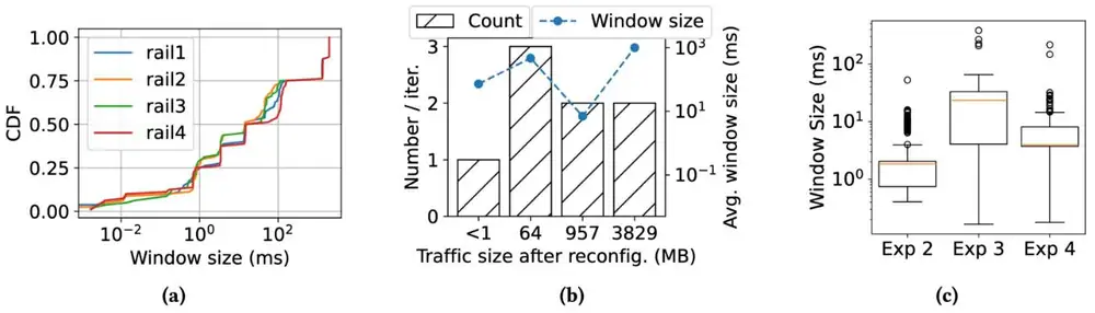
In panel (b), the eight windows of one iteration precede four kinds of operations: AllReduce synchronization calls under 1 MB (1 window), 64 MB PP Send/Recv (3), 957 MB DP AllGather (2) and the ReduceScatter (2). The paper's simulations add that windows shrink as data parallelism grows at a fixed global batch; we do not report those simulated sizes.
在 (b) 中,一次迭代的八個窗口分別位於四種操作之前:小於 1 MB 的 AllReduce 同步呼叫(1 個窗口)、64 MB 的 PP Send/Recv(3 個)、957 MB 的 DP AllGather(2 個)與 ReduceScatter(2 個)。論文的模擬補充:全域 batch 固定而資料平行度增加時,窗口會縮短;我們不報告那些模擬出的大小。
The design設計
1. Time-multiplex the ports across phases1. 在階段之間分時共用埠
Since phases do not overlap, the same NIC ports can serve every dimension in turn. At each phase boundary Opus re-wires the rail's OCS into the circuits that the next collective needs, typically a ring, which needs degree 2. Each phase then gets the full NIC bandwidth, and the number of parallelisms no longer depends on the port count. TP stays inside the scale-up domain and never touches the rail. The delay that communication sees is
既然階段不重疊,同一組 NIC 埠就能輪流服務每個維度。在每個階段邊界,Opus 把 rail 的 OCS 重新接成下一個集體操作需要的電路,通常是一個 ring,只需要度數 2。於是每個階段都拿到完整的 NIC 頻寬,平行化維度的數量也不再受埠數限制。TP 留在 scale-up 網域內,從不經過 rail。通訊看到的延遲是
if each switch starts at the beginning of its window. This is provisioning: the shim requests the next phase's circuits as soon as the last operation of the current phase completes. Without it, the switch starts only when the next operation arrives, and every switch is exposed in full.
前提是每次切換都在窗口開頭就開始。這就是預先配置(provisioning):當前階段最後一個操作一完成,shim 就請求下一階段的電路。沒有它,切換要等下一個操作到來才開始,每次切換都完整外露。
2. Shim, controller, orchestrator2. Shim、控制器、編排器
A per-rank shim intercepts every collective and reads its group, type and size. It decides three things: whether the operation uses the GPU network or the CPU front-end network (barriers and small calls), whether a phase boundary is reached, and whether to switch on demand or by provisioning. It then issues a blocking topo_write. A per-job controller acts as a barrier: when all ranks of a group have asked, it updates the rail's topo_id, forwards it to the orchestrators, waits for their acknowledgements and releases the ranks. A per-rail orchestrator programs the OCS through a vendor-neutral driver. The topo_id has one decimal digit per PP stage: 0 means that PP owns the stage's circuits, and 1, 2, … name a symmetric parallelism such as DP or CP. The orchestrator stores one sub-mapping per stage and reprograms only the stages whose digit changed:
每個 rank 一個 shim,攔截每個集體操作,讀出它的群組、類型與大小。它決定三件事:這個操作走 GPU 網路還是 CPU 前端網路(barrier 與小呼叫走後者)、是否到了階段邊界,以及要按需切換還是預先配置。接著它發出阻塞式的 topo_write。每個任務一個控制器,扮演 barrier:一個群組的所有 rank 都提出請求後,它更新該 rail 的 topo_id、轉給編排器、等待確認,再放行各 rank。每條 rail 一個編排器,透過與廠商無關的驅動程式設定 OCS。topo_id 每個 PP 階段一位十進位數字:0 表示該階段的電路歸 PP,1、2、… 代表 DP 或 CP 之類的對稱平行化。編排器為每個階段存一份子對應表,只重新設定數字有變的階段:
3. Safety and speed rules3. 安全與速度規則
Two guarantees come from a lock in the network backend: no operation runs on a topology being reconfigured (G1), and no reconfiguration starts while an operation is in flight on the affected sub-mappings (G2). Two optimizations follow. During the first ~5 training steps the shim records the sequence of collectives into a phase table; afterwards it switches only at phase boundaries and skips switches between operations of the same dimension (O1). Provisioning hides the switch in the window (O2). Pipeline parallelism is the exception. It is asymmetric: different stages run different phases at the same time, so Opus handles PP per operation. Each Send/Recv triggers topo_write from both stages and changes at most two digits. On a timeout, Opus retries; on persistent failure it falls back to one static "giant ring" through all ranks and notifies the framework.
網路後端的一把鎖提供兩項保證:拓樸重新配置時不執行任何操作(G1);受影響的子對應表上有操作在進行時,不開始重新配置(G2)。接著是兩項最佳化。在最初約 5 個訓練步中,shim 把集體操作的順序記進階段表;之後只在階段邊界切換,同一維度的連續操作之間不切換(O1)。預先配置把切換藏進窗口(O2)。管線平行是例外。它是非對稱的:不同階段在同一時間執行不同的階段,所以 Opus 對 PP 逐個操作處理。每次 Send/Recv 由兩個階段各發出 topo_write,最多改變兩位數字。逾時時 Opus 會重試;持續失敗時改用一條穿過所有 rank 的靜態「巨型 ring」,並通知框架。
4. All-to-all on a matching4. 在配對上做 all-to-all
Expert parallelism needs many peers at once. Opus gives each rail a different ring order over the scale-up domains of an EP group of size , where is the number of rails (GPUs per domain). Traffic first moves over NVLink to the rail whose ring links the two domains. The fraction of domain pairs that are one optical hop apart is bounded by
專家平行同時需要很多對端。Opus 讓每條 rail 在大小為 的 EP 群組的 個 scale-up 網域上使用不同的 ring 順序,其中 是 rail 數(每個網域的 GPU 數)。流量先經 NVLink 移到某條 rail,而那條 rail 的 ring 正好連著這兩個網域。相距一個光學跳躍的網域對比例上限為
so all pairs can be covered when : 10,440 GPUs for NVL72 domains (), by this analysis. A greedy algorithm picks each new rail's ring to cover the most new pairs. The results of this design come only from simulation.
所以當 時,所有網域對都能涵蓋:依此分析,NVL72 網域()可達 10,440 顆 GPU。貪婪演算法為每條新 rail 挑選能涵蓋最多新網域對的 ring。這個設計的結果只來自模擬。
Implementation實作
Opus is a custom PyTorch distributed backend: backend="opus" in init_process_group, or one flag in TorchTitan. It intercepts calls through ProcessGroup and delegates the transport to NCCL, so model and parallelism code do not change. The shim runs two threads: the main thread checks boundaries before dispatch, and a callback thread runs the provisioning step when the CUDA stream signals completion. The orchestrator speaks TL1, SCPI or NETCONF, so the same controller drives a real OCS or an emulator. The code is about 4,000 lines of C++ (PyTorch 2.10.0, NCCL 2.28, CUDA 12.8) plus a 300-line Python TL1 orchestrator, and it is open source. This digest uses the accepted ACM version. The arXiv v2 text differs: it gives ≈200 ms instead of ≈25 ms for the Polatis switch and lacks the cost model and the all-to-all design.
Opus 是一個自訂的 PyTorch 分散式後端:在 init_process_group 中設 backend="opus",或在 TorchTitan 中開一個旗標。它透過 ProcessGroup 攔截呼叫,把傳輸交給 NCCL,所以模型與平行化程式碼都不用改。shim 有兩個執行緒:主執行緒在送出前檢查邊界,回呼執行緒在 CUDA stream 回報完成時執行預先配置。編排器支援 TL1、SCPI 或 NETCONF,所以同一個控制器可以驅動真實 OCS 或模擬器。程式約 4,000 行 C++(PyTorch 2.10.0、NCCL 2.28、CUDA 12.8),外加 300 行 Python 的 TL1 編排器,並已開源。本導讀依據的是 ACM 接受版。arXiv v2 的內容不同:Polatis 交換器寫的是約 200 ms 而非約 25 ms,也沒有成本模型與 all-to-all 設計。
What was measured量到了什麼
A real optical testbed真實的光學測試平台
One Polatis Series 6000 OCS (64 ports) connects 4 servers, each with 2 L40 GPUs and 2 ConnectX-6 Dx NICs of two 100G ports: 16 transceivers and 32 fibers wired as 2 rails. RoCEv2, the Mellanox driver and NCCL 2.28 run unmodified; only the RDMA retry count is set to 7, so that queue pairs survive a switch and NCCL reuses its connections. A 6-layer Llama-3 trains with DP2, TP2 and PP2, with TP over PCIe. Opus switched each rail 4 times per step between DP and PP circuits, and each phase got the full 200 Gb/s per GPU. Figure 9 of the paper times one switch:
一台 Polatis Series 6000 OCS(64 埠)連接 4 台伺服器,每台有 2 顆 L40 GPU 與 2 張雙 100G 埠的 ConnectX-6 Dx NIC:共 16 個光模組與 32 條光纖,接成 2 條 rail。RoCEv2、Mellanox 驅動程式與 NCCL 2.28 都未修改;只把 RDMA 重試次數設成 7,讓 queue pair 撐過切換、NCCL 能沿用連線。訓練的是 6 層的 Llama-3,DP2、TP2、PP2,TP 走 PCIe。Opus 每個步讓每條 rail 在 DP 與 PP 電路之間切換 4 次,每個階段都拿到每顆 GPU 完整的 200 Gb/s。論文的 Figure 9 量測一次切換的時間:
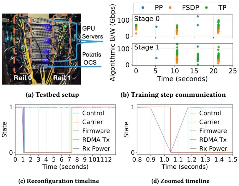
| Step after the switch command (real hardware)切換指令之後的步驟(真實硬體) | Measured time實測時間 |
|---|---|
| Optical Rx power back to baseline (ethtool samples every 100 ms)光 Rx 功率恢復基準(ethtool 每 100 ms 取樣) | within ≈ 200 ms≈ 200 ms 內 |
| NIC and transceiver firmware reports link-upNIC 與光模組韌體回報 link-up | ≈ 6 s; ≈ 3 s with auto-negotiation off≈ 6 s;關閉自動協商 ≈ 3 s |
| Linux netdev carrier flips, after firmware link-up韌體 link-up 之後 Linux netdev carrier 切換 | ≈ 70–80 µs |
| RDMA traffic resumes, after that之後 RDMA 流量恢復 | ≈ 100–200 ms more再 ≈ 100–200 ms |
So on real hardware the firmware, not the mirrors, set the switch time. The authors call this non-fundamental: the firmware treats a link change as a rare failure. With fast link-up, a switch would take the OCS time, ≈25 ms for their Polatis.
所以在真實硬體上,決定切換時間的是韌體,不是鏡面。作者認為這不是根本限制:韌體把鏈路變化當成罕見的故障。若 link-up 夠快,一次切換只需 OCS 的時間,他們的 Polatis 約 25 ms。
Real GPUs, emulated optical switch真實 GPU、模擬的光交換器
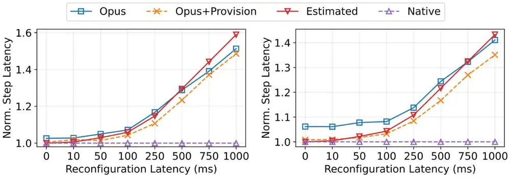
To test at larger scale without the firmware delay, the authors ran on Perlmutter's real A100 GPUs, NVLink and Slingshot-11 network, with the OCS emulated in software. Logical circuit switches enforce one-to-one connectivity and inject a chosen switching delay; the shim and controller run unmodified. Each result is the mean of 5 steps after 5 warm-up steps. Config. 1 is Llama-3-8B on 16 GPUs (TP4, FSDP2, PP2) and Config. 2 the same model on 64 GPUs (TP4, FSDP8, PP2); both need 6 switches per step. Every number in this table comes from that emulated-OCS setup:
為了在不受韌體延遲影響的情況下測試更大規模,作者在 Perlmutter 的真實 A100 GPU、NVLink 與 Slingshot-11 網路上執行,而 OCS 由軟體模擬。邏輯電路交換器強制一對一連線並注入指定的切換延遲;shim 與控制器未修改。每個結果是 5 個暖身步之後 5 個步的平均。Config. 1 是 16 顆 GPU 上的 Llama-3-8B(TP4、FSDP2、PP2),Config. 2 是 64 顆 GPU 上的同一模型(TP4、FSDP8、PP2);兩者每步都需要切換 6 次。下表每個數字都來自這個模擬 OCS 的設定:
| Question (real GPUs and network, emulated OCS)問題(真實 GPU 與網路、模擬 OCS) | Calculation算式 | Result結果 |
|---|---|---|
| Step time at a 50 ms emulated switch, Configs. 1 / 2, without provisioning (Figure 10)模擬切換 50 ms 時的步時間,Config. 1/2,不預先配置(Figure 10) | relative to native相對於原生 | / |
| Same with provisioning同上,預先配置 | relative to native相對於原生 | / |
| Control overhead at a 0 ms emulated switch, Config. 2 (64 GPUs): native 13.86 s, Opus 14.71 s模擬切換 0 ms 時的控制開銷,Config. 2(64 顆 GPU):原生 13.86 s、Opus 14.71 s | +6.13%+6.13% | |
| Same with provisioning: 13.97 s同上,預先配置:13.97 s | +0.79%+0.79% | |
| PP-only Config. 3 (DeepSeek-V3-16B): native 7.28 s, Opus 7.75 s at 0 ms and 7.76 s at 100 ms只有 PP 的 Config. 3(DeepSeek-V3-16B):原生 7.28 s,Opus 0 ms 時 7.75 s、100 ms 時 7.76 s | +6.46%, no switch at all+6.46%,完全沒有切換 |
Provisioning matters most for Config. 2, whose larger DP groups wait longer for their slowest rank and so leave wider windows. Without switching, the overhead is the control path: per-rail locking and rank synchronization through the controller. Provisioning hides most of it in the windows. In Config. 3, all scale-out traffic is PP, so Opus suppresses every switch, and the 6.46% is the per-operation PP control messages. The emulation cannot show the congestion-free benefit of optical links, and its baseline is Slingshot-11, not a rail-optimized fabric.
預先配置對 Config. 2 最重要:它的 DP 群組較大,等最慢 rank 的時間較長,窗口也就較寬。沒有切換時,開銷來自控制路徑:每條 rail 的鎖與透過控制器的 rank 同步。預先配置把大部分開銷藏進窗口。Config. 3 的 scale-out 流量全是 PP,所以 Opus 抑制了所有切換,6.46% 是逐操作 PP 控制訊息的成本。模擬無法呈現光鏈路沒有壅塞的好處,基準也是 Slingshot-11,而不是 rail-optimized 網路。
Simulation and the cost model模擬與成本模型
Results at 128–2,048 GPUs, the expert-parallel experiment and the frontier-scale windows come from ASTRA-sim simulation, so we do not report them. Cost and power come from a per-port model, with the same form for power and fibers excluded. Opus needs no switch ports, 2 OCS ports and 1 transceiver per GPU; a pluggable electrical fabric needs a transceiver per GPU and per switch port. For H200 clusters at 400G (64–512 GPUs), the model gives Opus 4.3× lower cost and 23.9× lower power than a rail-optimized electrical fabric; for B200 with co-packaged-optics switches (512–2,048 GPUs), 3.2× and 15.4×. One port's values show why power falls more than cost (Table 2 inputs, our arithmetic):
128–2,048 顆 GPU 的結果、專家平行實驗與前沿規模的窗口都來自 ASTRA-sim 模擬,所以我們不報告。成本與功耗來自逐埠模型 功耗同形式,不含光纖。Opus 每顆 GPU 不需交換器埠,需要 2 個 OCS 埠與 1 個光模組;可插拔光模組的電子網路則每顆 GPU 與每個交換器埠都要一個光模組。對 400G 的 H200 叢集(64–512 顆 GPU),模型給出 Opus 比 rail-optimized 電子網路成本低 4.3 倍、功耗低 23.9 倍;對使用共封裝光學交換器的 B200(512–2,048 顆 GPU),則是 3.2 倍與 15.4 倍。一個埠的數值說明為何功耗降得比成本多(Table 2 的輸入,我們的計算):
| Question (cost-model inputs, H200, 400G)問題(成本模型輸入,H200、400G) | Calculation算式 | Result結果 |
|---|---|---|
| Power of one electrical port with its transceiver, against one OCS port一個電子埠加其光模組的功耗,對一個 OCS 埠 | ||
| Price of the same, against one OCS port同樣的價格,對一個 OCS 埠 |
An OCS port costs almost as much as a switch port but draws about 100× less power, and the GPU-side transceivers ($719 and 10 W each) stay in both designs. All of these ratios are model outputs, not measurements.
OCS 埠的價格與交換器埠差不多,功耗卻低約 100 倍,而 GPU 端的光模組(每個 $719、10 W)兩種設計都保留。這些比例全是模型輸出,不是量測值。
Panel 1 lets you test a switch time against the measured windows.
面板 1 讓你拿一個切換時間去對照實測的窗口。
Limits and open questions限制與未解問題
- The NIC, not the mirror. On real hardware, the seconds-long NIC and transceiver re-link, not the optical switch, set the reconfiguration time, and the paper left it out of its timing: the testbed showed only that the mechanism works, and the step-time results use an emulated OCS that injects only the switching delay. MixNet measured the same effect with other NICs (5.67 s on average) and also excluded it from its timing. Both groups call it firmware and optics engineering, not physics, but until fast link-up ships, a photonic rail stops for seconds at every phase boundary.問題在 NIC,不在鏡面。在真實硬體上,決定重新配置時間的是長達數秒的 NIC 與光模組重新連線,而不是光交換器,而論文的計時沒有算進去:測試平台只證明機制可行,步時間結果用的是只注入切換延遲的模擬 OCS。MixNet 用不同的 NIC 量到同樣的現象(平均 5.67 s),也同樣把它排除在計時之外。兩組作者都說這是韌體與光學的工程問題,不是物理限制;但在快速 link-up 上市前,光子 rail 在每個階段邊界都會停數秒。
- Small measured scale. The optical testbed has 8 GPUs on 2 rails, and the emulation reaches 64 GPUs. Windows measured on 16–64 GPUs may shrink at large scale, which the paper shows only in simulation.實測規模小。光學測試平台只有 2 條 rail 上的 8 顆 GPU,模擬最多到 64 顆。在 16–64 顆 GPU 上量到的窗口在大規模時可能縮短,而論文只用模擬呈現這一點。
- Rings only. A degree-2 circuit gives up trees and recursive doubling, which win for small messages; the cost of that choice is not isolated. All-to-all needs the divergent rings and NVLink forwarding, evaluated only in simulation.只能用 ring。度數 2 的電路放棄了在小訊息時較佳的 tree 與 recursive doubling;這個選擇的代價沒有單獨量測。all-to-all 需要分歧 ring 與 NVLink 轉送,只在模擬中評估。
- A stable schedule. The phase table assumes that every iteration repeats the same collectives. Variable sequence lengths, data-dependent MoE routing and other jobs sharing the rail are discussed but not measured. PP still costs about 6.5% in control messages.穩定的排程。階段表假設每次迭代重複同樣的集體操作。可變序列長度、依資料而定的 MoE 路由,以及其他任務共用 rail 的情況都只有討論、沒有量測。PP 的控制訊息仍約花 6.5%。
- Model prices. The 4.3× and 23.9× come from per-port list prices and power figures, without fiber, cabling or labour.模型價格。4.3 倍與 23.9 倍來自逐埠的牌價與功耗數字,不含光纖、佈線與人工。
How it connects與其他內容的關聯
Opus keeps the rail wiring of HPN, Llama 3 and rail-only, and uses rail-only's NVLink forwarding for cross-rail traffic. It moves TPU v4's OCS from per-job to per-phase reconfiguration. Its phases are the ones of Section 3.8, and its ring-only limit relates to the ring-versus-tree trade-off in Section 4.3. MixNet switches inside the EP phase on a regional OCS next to an electrical fabric; Opus switches between phases on an all-optical rail. Harvest goes one timescale down, switching a photonic scale-up fabric between the steps of one collective, while ZCube and BST answer the same cost question with static electrical wiring.
Opus 保留 HPN、Llama 3 與 rail-only 的 rail 接線,並沿用 rail-only 的 NVLink 轉送處理跨 rail 流量。它把 TPU v4 的 OCS 從每任務一次推進到每階段重新配置。它的階段就是第 3.8 節的那些階段,而只能用 ring 的限制則關係到第 4.3 節的 ring 與 tree 取捨。MixNet 在 EP 階段之內、於電子網路旁的區域 OCS 上切換;Opus 在階段之間、於全光的 rail 上切換。Harvest 再往下一個時間尺度,在一次集體操作的各步之間切換光子 scale-up 網路;ZCube 與 BST 則用靜態電子接線回答同樣的成本問題。
Key numbers關鍵數字
| Number數字 | What it is, and how it was obtained是什麼、怎麼得到 |
|---|---|
| > 75% | Windows longer than 1 ms; Exp. 1 on Perlmutter, measured長於 1 ms 的窗口;Perlmutter 上的實驗 1,實測 |
| ≈ 1,000 ms | Mean window before the 3,829 MB ReduceScatter; same run3,829 MB ReduceScatter 之前的平均窗口;同一實驗 |
| 4 per step · 200 Gb/s | Switches per step and per-GPU bandwidth per phase; real optical testbed每步切換次數與每階段每顆 GPU 的頻寬;真實光學測試平台 |
| ≈ 6 s / ≈ 3 s | NIC firmware link-up, auto-negotiation on / off; real testbedNIC 韌體 link-up,自動協商開/關;真實測試平台 |
| ≈ 25 ms | Polatis switching time stated in the accepted paper (arXiv v2: ≈ 200 ms)接受版論文所寫的 Polatis 切換時間(arXiv v2:≈ 200 ms) |
| 1.01× / 1.02× | Step time at a 50 ms switch with provisioning, Configs. 1 / 2; real GPUs, emulated OCS50 ms 切換且預先配置時的步時間,Config. 1/2;真實 GPU、模擬 OCS |
| 13.86 / 14.71 / 13.97 s | Native / Opus / Opus with provisioning at 0 ms, 64 GPUs; real GPUs, emulated OCS0 ms 時原生/Opus/Opus 加預先配置,64 顆 GPU;真實 GPU、模擬 OCS |
| 4.3× / 23.9× | Lower cost / power than an electrical rail fabric, H200 at 400G; cost model比電子 rail 網路低的成本/功耗,400G 的 H200;成本模型 |
| ≈ 4,000 + 300 lines | C++ shim and controller, Python TL1 orchestratorC++ 的 shim 與控制器、Python 的 TL1 編排器 |
Terms used on this page本頁用到的術語
- Photonic rail
- A rail built from one OCS instead of packet switches.
- 以一台 OCS 而非封包交換器構成的 rail。
- Matching
- One-to-one port pairs: all the connectivity an OCS gives at one time.
- 一對一的埠配對:OCS 在某一時刻能提供的全部連線。
- Window
- Idle time between the last collective of one phase and the first of the next.
- 一個階段最後一個集體操作與下一階段第一個集體操作之間的閒置時間。
- Provisioning
- Requesting the next phase's circuits as soon as the current phase ends.
- 當前階段一結束就請求下一階段的電路。
- topo_id
- A per-rail number with one digit per PP stage, naming who owns that stage's circuits.
- 每條 rail 一個數字,每個 PP 階段一位,表示該階段的電路歸誰。
- Phase table
- The profiled order of collectives, used to detect phase boundaries.
- 剖析得到的集體操作順序,用來偵測階段邊界。
- Auto-negotiation
- The link-up procedure in which two ports agree on speed and mode; turning it off halved the link-up time.
- 兩個埠協商速率與模式的 link-up 程序;關掉它讓 link-up 時間減半。