Research digest 5 of 5 · Chapter 6: Topology

研究導讀 5 / 5 · 第 6 章：拓樸

Harvest: Adaptive Photonic Switching Schedules for Collective Communication in Scale-up DomainsHarvest：在 scale-up 域中為集體通訊自適應安排光子交換的時程

SIGCOMM 2026Mahir Rahman, Samuel Joseph, Nihar Kodkani, Behnaz Arzani, Vamsi Addanki (Purdue University, Microsoft Research) · paper論文

After reading, you can explain when a photonic scale-up fabric should re-wire during one collective, how Harvest's dynamic program finds the steps, and why rings never gain.讀完後，你能說明光子 scale-up 網路在一次集體操作中何時該重新接線、Harvest 的動態規劃如何找出那幾步，以及為何環演算法永遠得不到好處。

≈ 11 min · 1 interactive panel · 5-question quiz≈ 11 分鐘 · 1 個互動面板 · 5 題測驗Chapter 6 ↗第 6 章 ↗Jump to the quiz ↓跳到測驗 ↓

If you read nothing else

只讀這一段也可以

A photonic circuit switch can give every pair of GPUs a direct optical path. Each change of circuits costs a reconfiguration delay $\alpha_r$ : about 10 ns with tunable lasers, about 10 ms with 3-D MEMS mirrors. A collective runs in steps with known peers, and Harvest decides before which steps the circuits change. Its cost model is the α–β model plus propagation and congestion. A dynamic program picks the cut points, and a subproblem picks one topology for each run of steps. For recursive doubling the best topology for a run is the direct links of its first step, so no solver is needed; rings never gain from re-wiring. No photonic switch was used: the 8-GPU "hardware emulation" pauses NCCL between steps and adds a constant per reconfiguration. Measured: a per-hop $\alpha$ of 30.32 µs and $\beta$ of 85.11 Gb/s, schedule synthesis within 20 µs up to 64 GPUs, and GPU synchronization of about 4 µs for 8 GPUs. All speedups are simulation, so this page teaches the model.

光子電路交換器可以讓每一對 GPU 都有一條直接的光路徑。每次改變電路都要付出重新配置延遲 $\alpha_r$ ：可調雷射約 10 ns，3-D MEMS 鏡片約 10 ms。集體操作分成數個步驟、每步的夥伴事先已知，Harvest 決定在哪幾步之前改變電路。它的成本模型是 α–β 模型再加上傳播延遲與壅塞。動態規劃挑選切點，子問題為每一段連續步驟挑選一個拓樸。對遞迴倍增而言，一段步驟的最佳拓樸就是其第一步的直接鏈路，所以不需要求解器；環演算法則永遠不會因重新接線而受益。論文沒有用到任何光子交換器：8 GPU 的「硬體模擬」在步驟之間暫停 NCCL，並為每次重新配置加上一個常數。實測的是：每跳 $\alpha$ 為 30.32 µs、 $\beta$ 為 85.11 Gb/s，64 顆 GPU 以內的排程合成在 20 µs 內完成，8 顆 GPU 的同步約 4 µs。所有加速倍數都來自模擬，所以本頁教的是模型。

1. Where this paper sits1. 這篇論文的位置

The Chapter 4 (section 2, Panel 2) prices a collective as $\alpha$ per dependent step plus bytes over bandwidth. The ring takes $2(N-1)$ steps and sends the fewest bytes; recursive doubling takes $\log_2 N$ steps and sends more. Both formulas assume that peers talk at full rate. On a fixed ring this is false for recursive doubling: in step $i$ the peers are $2^{i-1}$ hops apart, so $2^{i-1}$ flows share each link. Harvest adds a third option: change the wiring.

第 4 章（第 2 節，面板 2）把一次集體操作的成本算成每個相依步驟一個 $\alpha$ ，再加上位元組除以頻寬。環要 $2(N-1)$ 步、送出的位元組最少；遞迴倍增只要 $\log_2 N$ 步，但送得較多。兩條公式都假設夥伴之間以全速通訊。在固定的環上，這對遞迴倍增並不成立：第 $i$ 步的夥伴相隔 $2^{i-1}$ 跳，所以每條鏈路上有 $2^{i-1}$ 條流共用。Harvest 加入第三種選擇：改變接線。

The Chapter 6 (section 5, Panel 5) shows TPU v4, where optical circuit switches (OCS) re-wire a torus once per job. Two digests of this chapter re-wire during training, in milliseconds, in the scale-out network: MixNet inside each MoE layer and Opus between parallelism phases. Harvest works inside one collective, in a scale-up domain of 8 to 64 GPUs, where photonic switches can change in nanoseconds to microseconds.

第 6 章（第 5 節，面板 5）介紹 TPU v4：光電路交換器（OCS）每個任務重新接線一次環面。本章另有兩篇導讀在訓練進行中、在 scale-out 網路裡以毫秒級重新接線：MixNet 在每個 MoE 層內，Opus 在平行化階段之間。Harvest 則在單一次集體操作內運作，範圍是 8 到 64 顆 GPU 的 scale-up 域，那裡的光子交換器可以在奈秒到微秒內切換。

What was missing. Earlier circuit schedulers decompose an aggregate traffic matrix and assume that all of its demand is available at once, or they ignore $\alpha_r$ . In a collective, the data of step $i+1$ exists only after step $i$ . Topology-aware algorithms (Swing, Bruck) and collective synthesis (TE-CCL) fix the topology and search the schedule. Harvest is the converse: it fixes the schedule and searches a topology for each step.

過去缺少什麼。先前的電路排程器把總流量矩陣拆解，並假設其中所有需求同時就緒；或是乾脆忽略 $\alpha_r$ 。在集體操作中，第 $i+1$ 步的資料要等第 $i$ 步完成才存在。拓樸感知演算法（Swing、Bruck）與集體操作合成（TE-CCL）固定拓樸、搜尋排程。Harvest 正好相反：固定排程，為每一步搜尋拓樸。

2. The problem, in the paper's example2. 問題：論文的例子

The paper has no measurement study. Its motivation is a worked example (§3.2): recursive doubling on 8 GPUs, in the cyclic variant where GPU $j$ sends to GPU $j + 2^{i-1} \bmod 8$ in step $i$ .

論文沒有量測研究，它的動機是一個算例（§3.2）：8 顆 GPU 上的遞迴倍增，採循環版本，在第 $i$ 步 GPU $j$ 送給 GPU $j + 2^{i-1} \bmod 8$ 。

Six ring diagrams of 8 GPUs: three steps on the static ring with congestion 1, 2 and 4, and the same steps after re-wiring to distance-2 and distance-4 circuits — Figure 2 of the paper (a diagram, not data). Black lines are circuits; red arrows are the step's transfers. Top: the static ring $G_1$ , where steps 1–3 have congestion 1, 2 and 4. Bottom: after re-wiring to $G_2$ (GPUs two apart joined) and $G_3$ (four apart). Panel (c) is labelled $G_3$ in the paper but shows step 3 on the ring $G_1$ .論文圖 2（示意圖，不是資料）。黑線是電路，紅色箭頭是該步的傳輸。上排：靜態環 $G_1$ ，第 1–3 步的壅塞為 1、2、4。下排：重新接線成 $G_2$ （相隔兩個的 GPU 相連）與 $G_3$ （相隔四個）之後。論文把 (c) 標為 $G_3$ ，但它畫的是環 $G_1$ 上的第 3 步。Rahman et al., SIGCOMM 2026, Figure 2 (accepted version).

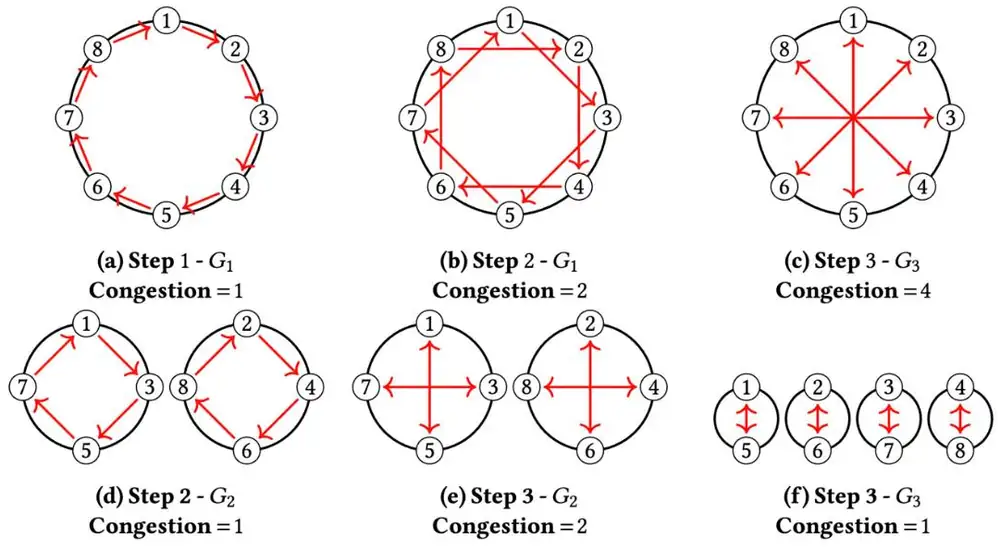
If the circuits change before step 2 to join GPUs two apart, step 2 has congestion 1 and step 3 has 2. A second change before step 3 makes every step direct. The paper's Table 1 compares the three schedules, relative to the best:

如果在第 2 步之前把電路改成連接相隔兩個的 GPU，第 2 步的壅塞變成 1，第 3 步為 2。在第 3 步之前再改一次，每一步都變成直接連線。論文的 Table 1 比較這三種排程（相對於最佳值）：

Circuits in steps 1, 2, 3第 1、2、3 步的電路	Congestion壅塞	Propagation傳播	Reconfigurations重新配置
$G_1, G_1, G_1$ (static)（靜態）	4×	4×	0
$G_1, G_2, G_2$	2×	2×	1
$G_1, G_2, G_3$ (every step)（每一步）	1×	1×	2

Re-wiring before every step is a BvN schedule. It wins when $\alpha_r$ is small; the static ring wins when $\alpha_r$ is large. Harvest is about the schedules between them.

每一步之前都重新接線稱為 BvN 排程。 $\alpha_r$ 小時它勝出； $\alpha_r$ 大時靜態環勝出。Harvest 處理的是兩者之間的排程。

3. The design3. 設計

3.1 The cost of one step on one topology3.1 一個步驟在一個拓樸上的成本

Step $i$ moves $m_i$ bytes along the pattern $\mathcal{M}_i$ , a 0/1 matrix of who sends to whom, on topology $G_i$ . The maximum concurrent flow $\theta(G_i, \mathcal{M}_i)$ is the largest fraction of the step's demand that the links carry at the same time, so $1/\theta$ is the congestion. The step's demand completion time is (Eq. 3)

第 $i$ 步在拓樸 $G_i$ 上依模式 $\mathcal{M}_i$ （記錄誰送給誰的 0/1 矩陣）搬運 $m_i$ 位元組。最大並行流 $\theta(G_i, \mathcal{M}_i)$ 是鏈路能同時承載的該步需求的最大比例，所以 $1/\theta$ 就是壅塞。該步的需求完成時間是（Eq. 3）

\begin{aligned} \mathrm{DCT}(m_i \mathcal{M}_i, G_i) &= \alpha + \delta\,\ell_i(G_i) \\ &\quad + \beta\,\frac{m_i}{\theta(G_i, \mathcal{M}_i)} \end{aligned}

Here $\alpha$ is the per-step setup latency, $\delta$ the propagation delay of one link, $\ell_i$ the longest path through the most congested links, and $\beta = 1/c$ for link capacity $c$ . With $\delta = 0$ and $\theta = 1$ this is Chapter 6's α–β model (Observation 2). The collective costs (Eq. 4)

其中 $\alpha$ 是每步的啟動延遲， $\delta$ 是一條鏈路的傳播延遲， $\ell_i$ 是經過最壅塞鏈路的最長路徑， $\beta = 1/c$ ， $c$ 是鏈路容量。當 $\delta = 0$ 且 $\theta = 1$ ，這就是第 6 章的 α–β 模型（Observation 2）。整個集體操作的成本是（Eq. 4）

\begin{aligned} t_c(1,s) = \sum_{i=1}^{s} \Big( &\alpha + \delta\,\ell_i(G_i) + \beta\,\frac{m_i}{\theta(G_i,\mathcal{M}_i)} \\ &+ \alpha_r\,\mathbb{I}(E_i \ne E_{i-1}) \Big) \end{aligned}

The last term charges $\alpha_r$ whenever the link set $E_i$ changes. In point-to-point algorithms each $\mathcal{M}_i$ is a permutation, so a collective is a Birkhoff–von Neumann (BvN) decomposition of its total demand, with an order fixed by data dependencies (Observation 1).

最後一項在鏈路集合 $E_i$ 改變時收取 $\alpha_r$ 。在點對點演算法中每個 $\mathcal{M}_i$ 都是排列，所以一次集體操作就是其總需求的 Birkhoff–von Neumann（BvN）分解，只是順序由資料相依性固定（Observation 1）。

3.2 One topology for a run of steps3.2 為一段連續步驟選一個拓樸

The subproblem takes steps $a$ to $b$ with no re-wiring inside and finds the one topology $G_{a,b}$ that minimizes their summed time (Eqs. 5–6). Appendix A writes it as a mixed-integer second-order cone program (MISOCP). An integer $x_{u,v}$ counts links from $u$ to $v$ , at most $d$ per node; each step's flows carry $\theta_i$ of its demand within capacity $c\,x_{u,v}$ ; and time obeys $\theta_i T_i \ge \beta m_i$ , a cone constraint. The cone appears because one topology serves several demands one after another; with all demand at once it would be a linear program. The MISOCP is solvable up to about 64 GPUs. The evaluation restricts candidates to shifted rings, an expander, shifted tori and the per-step matchings, which removes the integers.

子問題取第 $a$ 到第 $b$ 步、中間不重新接線，找出使這些步驟總時間最小的單一拓樸 $G_{a,b}$ （Eqs. 5–6）。附錄 A 把它寫成混合整數二階錐規劃（MISOCP）。整數 $x_{u,v}$ 計算從 $u$ 到 $v$ 的鏈路數，每個節點最多 $d$ 條；每一步的流在容量 $c\,x_{u,v}$ 之內承載該步需求的 $\theta_i$ ；時間滿足 $\theta_i T_i \ge \beta m_i$ ，這是一個錐限制。錐的出現是因為同一個拓樸要先後服務好幾個需求；若所有需求同時存在，它就只是線性規劃。MISOCP 可解到約 64 顆 GPU。評估時把候選限制為平移環、一個擴展圖、平移環面與各步的配對，於是整數變數消失。

3.3 When to re-wire: a dynamic program3.3 何時重新接線：動態規劃

$DP[a][k]$ is the best time from step $a$ to the end with exactly $k$ reconfigurations, without $\alpha_r$ . Lemma 1 splits at the first reconfiguration $b$ :

$DP[a][k]$ 是從第 $a$ 步到最後、恰好 $k$ 次重新配置的最佳時間，不含 $\alpha_r$ 。Lemma 1 在第一次重新配置的位置 $b$ 切開：

\begin{aligned} DP[a][k] &= \min_{a < b \le s+1} \big( t_c(a, b-1) \\ &\qquad + DP[b][k-1] \big) \\ DP[a][0] &= t_c(a, s) \end{aligned}

$\alpha_r$ is the same for every change, so Theorem 1 adds it at the end:

每次改變的 $\alpha_r$ 都相同，所以 Theorem 1 在最後才把它加上：

k^* = \arg\min_{k \in \{0,\dots,s\}} \big( DP[1][k] + k\,\alpha_r \big)

The schedule is optimal for the given algorithm. The cost is $O(s^4 g)$ , where $g$ is one subproblem. Schedules are computed offline and cached, off the critical path.

對給定的演算法，這個排程是最佳的。成本是 $O(s^4 g)$ ， $g$ 是一個子問題的成本。排程離線計算並快取，不在關鍵路徑上。

3.4 Recursive doubling and rings in closed form3.4 遞迴倍增與環的封閉形式

For recursive doubling two observations remove the solver (§5). Observation 3: direct links for step $i$ keep every later step connected, because the peer at distance $2^{j-1}$ is $2^{j-i}$ hops along them. Observation 4: for steps $a$ to $b$ , the best topology is the direct links of step $a$ ; later steps take 2, 4, … hops with equal congestion, the minimum. With $m/2^i$ bytes in step $i$ (reduce-scatter; the all-gather mirrors it), a run costs (Eq. 8)

對遞迴倍增，兩個觀察讓求解器變得多餘（§5）。Observation 3：為第 $i$ 步建立的直接鏈路讓之後每一步都保持連通，因為距離 $2^{j-1}$ 的夥伴沿這些鏈路走 $2^{j-i}$ 跳就到。Observation 4：對第 $a$ 到第 $b$ 步，最佳拓樸是第 $a$ 步的直接鏈路；之後的步驟走 2、4、… 跳，壅塞相同，都是最小值。第 $i$ 步送 $m/2^i$ 位元組時（reduce-scatter；all-gather 是它的鏡像），一段步驟的成本是（Eq. 8）

\begin{aligned} t_c(a,b) &= \alpha\,(b-a+1) + \delta\,\big(2^{\,b-a+1} - 1\big) \\ &\quad + \beta\, m\, \frac{b-a+1}{2^{a}} \end{aligned}

Each run is then $O(1)$ , and synthesis is $O((\log n)^4)$ . Appendix B proves the same for hypercube all-to-all, Bruck's algorithms, binomial-tree broadcast and Trivance. Appendix C.1 gives the rule: a cyclic pattern $u \to u+d$ whose distance grows geometrically. A ring algorithm uses the same ring in every step, so the observations make the static ring optimal (Appendix C.2): rings never gain from re-wiring. They pay with their number of steps instead.

於是每一段都是 $O(1)$ ，合成是 $O((\log n)^4)$ 。附錄 B 對 hypercube all-to-all、Bruck 的各演算法、二項樹廣播與 Trivance 證明了同樣的性質。附錄 C.1 給出規則：循環模式 $u \to u+d$ ，且距離呈等比成長。環演算法每一步都用同一個環，所以這些觀察使靜態環成為最佳（附錄 C.2）：環永遠不會因重新接線而受益，它付出的代價是步數。

Appendix C of the accepted version works this out for an all-gather on 64 GPUs: 6 steps of recursive doubling against 63 ring steps, with $m = 4$ MB, $\alpha = 500$ ns, $\delta = 50$ ns and 800 Gb/s. At $\alpha_r = 10$ µs the optimum re-wires twice. In the step order of Eq. 8 the runs are step 1, steps 2–3 and steps 4–6. The arithmetic, one question per row:

正式版附錄 C 以 64 顆 GPU 的 all-gather 算出這件事：遞迴倍增 6 步對環的 63 步， $m = 4$ MB、 $\alpha = 500$ ns、 $\delta = 50$ ns、800 Gb/s。 $\alpha_r = 10$ µs 時最佳排程重新接線兩次。依 Eq. 8 的步驟順序，三段是第 1 步、第 2–3 步與第 4–6 步。逐列計算如下：

Question問題	Calculation算式	Result結果
$\beta m$ : 4 MB at 800 Gb/s (100 GB/s) $\beta m$ ：4 MB、800 Gb/s（100 GB/s）	$4 \times 2^{20} \div 10^{11}$	$\approx 41.94$ µs
Run 1: step 1 on its direct links第 1 段：第 1 步，用自己的直接鏈路	$0.5 + 0.05 + 41.94 \div 2$	$\approx 21.52$ µs
Run 2: steps 2–3 on distance-2 links第 2 段：第 2–3 步，用距離 2 的鏈路	$2 \times 0.5 + 3 \times 0.05 + 41.94 \times 2/4$	$\approx 22.12$ µs
Run 3: steps 4–6 on distance-8 links第 3 段：第 4–6 步，用距離 8 的鏈路	$3 \times 0.5 + 7 \times 0.05 + 41.94 \times 3/16$	$\approx 9.71$ µs
Two reconfigurations兩次重新配置	$2 \times 10$	$20$ µs
Total總計	$21.52 + 22.12 + 9.71 + 20$	$\approx 73.36$ µsTable 1: 73,357.95 nsTable 1：73,357.95 ns

A smaller $\alpha_r$ re-wires more often: 5 times at 10 ns (44.64 µs) and 4 times at 1 µs (49.29 µs). The ring algorithm needs 75.94 µs and recursive doubling on the static ring 131.98 µs. Our implementation of Eq. 8 and the dynamic program reproduces every Table 1 value within 1 ns. Figure A shows where it cuts.

$\alpha_r$ 越小，重新接線越頻繁：10 ns 時 5 次（44.64 µs），1 µs 時 4 次（49.29 µs）。環演算法需要 75.94 µs，靜態環上的遞迴倍增需要 131.98 µs。我們依 Eq. 8 與動態規劃實作的模型，重現 Table 1 每個值的誤差都在 1 ns 以內。圖 A 畫出它切在哪裡。

Figure A shows the dynamic program's choice for the Appendix C example, in the step order of Eq. 8. Each shaded run uses the direct links of its first step; red bars are reconfigurations. As

\alpha_r

grows, runs merge and later steps pay 2 or 4 hops of congestion. Totals are from the model.圖 A 呈現附錄 C 例子中動態規劃的選擇，依 Eq. 8 的步驟順序。每個色塊段落使用其第一步的直接鏈路；紅色長條是重新配置。

\alpha_r

變大時段落合併，後面的步驟要付 2 或 4 跳的壅塞。總時間來自模型。Drawn for this primer from §5 and Appendix C (Table 1) of the paper.

Figure B splits the same schedules into the four terms of Eq. 4. It shows why each loser loses.

圖 B 把同樣的排程拆成 Eq. 4 的四項，說明每個輸家輸在哪裡。

Figure B, drawn from model values. The ring algorithm loses on

\alpha

(63 steps). Recursive doubling on the static ring loses on bytes times congestion. Harvest trades some congestion for a few

\alpha_r

.圖 B，依模型值繪製。環演算法輸在

\alpha

（63 步）。靜態環上的遞迴倍增輸在位元組乘以壅塞。Harvest 用幾次

\alpha_r

換掉一部分壅塞。Drawn for this primer from Eq. 4, Eq. 8 and Table 1 of the paper.

The panel runs Eq. 8 and the dynamic program for every message size and $\alpha_r$ . Its defaults are the measured testbed values.

下面的面板對每一種訊息大小與 $\alpha_r$ 執行 Eq. 8 與動態規劃。預設值是實測的測試平台數值。

Panel 1面板 1

When to re-wire: static ring, every step, or Harvest's choice (model)何時重新接線：靜態環、每一步，或 Harvest 的選擇（模型）

GPUs

n

GPU 數

n

Message size

m

訊息大小

m

Reconfiguration delay

\alpha_r

重新配置延遲

\alpha_r

Per-step setup

\alpha

每步啟動

\alpha

Link rate

1/\beta

鏈路速率

1/\beta

Propagation per link

\delta

每條鏈路的傳播

\delta

Presets預設組合

Harvest's reconfigurations

Harvest 的重新配置次數

Harvest time

Harvest 的時間

Static ring · every step

靜態環 · 每一步

Ring algorithm

環演算法

Model only: Eq. 8 for each run of steps and the dynamic program of Lemma 1 and Theorem 1, for the reduce-scatter (or mirrored all-gather) half of recursive doubling; the paper's simulated speedups are not shown. "Static ring" keeps the step-1 circuits; "every step" re-wires before each of the $\log_2 n - 1$ later steps; the ring algorithm takes $n-1$ steps of $m/n$ bytes on the ring. The map colors each cell by the fastest option, and the outlined cell is the slider setting. Defaults are the paper's measured testbed values: 8 GPUs, $\alpha = 30.32$ µs and $\beta$ of 85.11 Gb/s, with $\delta = 0$ because the measured $\alpha$ already includes the path. MB means $2^{20}$ bytes. The "Appendix C" preset reproduces Table 1: 73.36 µs with 2 reconfigurations, against 75.94 µs for the ring and 131.98 µs for the static ring; move $\alpha_r$ to 10 ns and 1 µs. Try more GPUs: more steps leave more room for selective schedules. Raise $\alpha_r$ past about 100 µs: re-wiring stops paying and, for large messages, the ring algorithm wins.

只有模型：對每段步驟用 Eq. 8，再用 Lemma 1 與 Theorem 1 的動態規劃，計算遞迴倍增的 reduce-scatter 半段（或其鏡像 all-gather）；不顯示論文的模擬加速。「靜態環」保留第 1 步的電路；「每一步」在其後 $\log_2 n - 1$ 步每一步之前都重新接線；環演算法在環上走 $n-1$ 步、每步 $m/n$ 位元組。地圖依最快的選項為每格上色，框起的格子是目前滑桿的設定。預設值是論文實測的測試平台：8 顆 GPU、 $\alpha = 30.32$ µs、 $\beta$ 為 85.11 Gb/s， $\delta = 0$ ，因為實測的 $\alpha$ 已包含路徑。MB 表示 $2^{20}$ 位元組。「附錄 C」預設組合重現 Table 1：73.36 µs、2 次重新配置，對照環的 75.94 µs 與靜態環的 131.98 µs；再把 $\alpha_r$ 移到 10 ns 與 1 µs 看看。試試更多 GPU：步數越多，選擇性排程的空間越大。把 $\alpha_r$ 提高到約 100 µs 以上：重新接線不再划算，訊息大時環演算法勝出。

4. Implementation4. 實作

The synthesizer is C++ and calls Gurobi for the cone subproblems. The authors extended the packet-level simulator Astra-Sim to follow a reconfiguration schedule and released both (github.com/STyGIANet/Harvest).

合成器以 C++ 寫成，錐子問題交給 Gurobi 求解。作者擴充封包層級模擬器 Astra-Sim，使它能依重新配置排程運作，並公開了兩者（github.com/STyGIANet/Harvest）。

The "hardware emulation" connects 8 GPUs in a ring through 8 BlueField-3 NICs with 100 Gb/s optical transceivers. GPUs reach their NICs by GPUDirect RDMA over PCIe, and the NICs route in the BlueField-3 eSwitch with hardware flow steering. NCCL runs the collective one step at a time. At each planned reconfiguration, execution pauses, the configuration is updated, and execution resumes. The reported time is the sum of the measured step times plus a fixed penalty for each reconfiguration. Nothing ran on a photonic switch: in every result, the reconfiguration delay is a constant that the authors add. There is no end-to-end training system.

「硬體模擬」用 8 張 BlueField-3 NIC 與 100 Gb/s 光模組把 8 顆 GPU 接成一個環。GPU 透過 PCIe 上的 GPUDirect RDMA 連到 NIC，NIC 之間在 BlueField-3 eSwitch 中以硬體 flow steering 轉送。NCCL 一次執行集體操作的一步。到了每個預定的重新配置點，執行暫停、更新配置、再繼續。回報的時間是實測各步時間的總和，加上每次重新配置一個固定的懲罰值。沒有任何東西在光子交換器上執行：每個結果中的重新配置延遲，都是作者加上去的常數。也沒有端到端的訓練系統。

5. What was measured5. 量測了什麼

Setup (§6.1): 8 to 64 GPUs with 2 to 6 ports each; 800 Gb/s per port in simulation, 100 Gb/s in the emulation; $\alpha$ , $\delta$ and $\alpha_r$ swept from 10 ns to 10 ms. Baselines are static topologies (ring, 2-D and 3-D tori, generalized Kautz graphs) and BvN schedules. The collectives are recursive doubling, Swing and Bruck all-reduce, direct and Bruck all-to-all, and tree broadcasts. The paper's speedups over both baselines come from packet simulation, numerical optimization and the emulation with an added delay, so this page does not list them.

設定（§6.1）：8 到 64 顆 GPU，每顆 2 到 6 個埠；模擬中每埠 800 Gb/s，模擬硬體中 100 Gb/s； $\alpha$ 、 $\delta$ 與 $\alpha_r$ 從 10 ns 掃到 10 ms。基線是靜態拓樸（環、二維與三維環面、廣義 Kautz 圖）與 BvN 排程。集體操作包括遞迴倍增、Swing 與 Bruck all-reduce，直接與 Bruck all-to-all，以及樹狀廣播。論文對兩種基線的加速倍數來自封包模擬、數值最佳化與加上延遲的硬體模擬，所以本頁不列出。

Three things were measured. First, the authors fitted the α–β model to single-hop GPU-to-GPU transfers on the testbed:

實際量測的有三件事。第一，作者用測試平台上單跳 GPU 對 GPU 的傳輸擬合 α–β 模型：

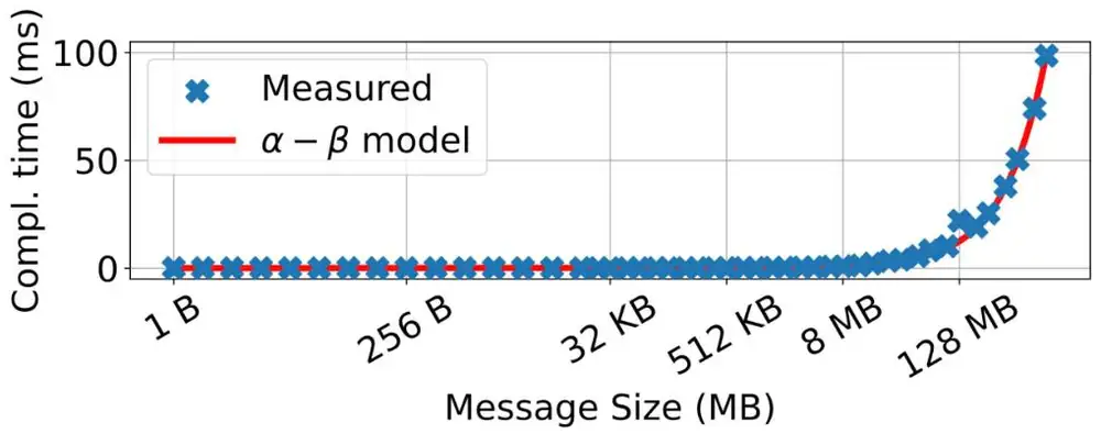
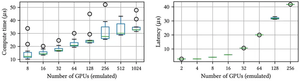
Measured completion time of one-hop transfers against message size, with the fitted alpha-beta line — Figure 7 of the paper (measured on the emulation testbed): completion time of single-hop transfers from 1 B to about 1 GB, with the fitted α–β line, $\alpha = 30.32$ µs and $\beta$ of 85.11 Gb/s. The axis says MB, but the ticks run from bytes to megabytes.論文圖 7（在模擬硬體測試平台上實測）：1 B 到約 1 GB 的單跳傳輸完成時間，以及擬合的 α–β 直線， $\alpha = 30.32$ µs、 $\beta$ 為 85.11 Gb/s。座標軸寫的是 MB，但刻度從位元組一路到 megabyte。Rahman et al., SIGCOMM 2026, Figure 7.

This $\alpha$ is about 60 times the 500 ns used in simulation, so the emulated regime is not the target regime. Second, the run time of the recursive-doubling dynamic program; third, the time for GPUs to synchronize through a shared-memory array before a step. Larger systems are emulated with more array entries and threads.

這個 $\alpha$ 約是模擬所用 500 ns 的 60 倍，所以模擬硬體所處的區間並不是目標區間。第二是遞迴倍增動態規劃的執行時間；第三是 GPU 在每步之前透過共享記憶體陣列同步所需的時間。更大的系統以更多陣列項目與執行緒來模擬。

Two box plots: synthesis compute time for 8 to 1024 GPUs, and synchronization latency for 2 to 256 GPUs — Figures 10 and 11 of the paper (measured). Left: run time of the recursive-doubling dynamic program, 8 to 1,024 GPUs. Right: synchronization latency through a shared-memory array, 2 to 256 GPUs; larger counts are emulated with threads.論文圖 10 與圖 11（實測）。左：遞迴倍增動態規劃的執行時間，8 到 1,024 顆 GPU。右：透過共享記憶體陣列的同步延遲，2 到 256 顆 GPU；較大的數量以執行緒模擬。Rahman et al., SIGCOMM 2026, Figures 10–11.

Quantity項目	Setup設定	Measured實測值
Per-hop $\alpha$ , $\beta$ 每跳 $\alpha$ 、 $\beta$	8 GPUs, BlueField-3 ring, 100G, NCCL8 顆 GPU、BlueField-3 環、100G、NCCL	30.32 µs · 85.11 Gb/s
Schedule synthesis排程合成	dynamic program, up to 64 / 1,024 GPUs動態規劃，至多 64 / 1,024 顆 GPU	≤ 20 µs · < 35 µs
GPU synchronizationGPU 同步	shared-memory array, 8 / 256 GPUs共享記憶體陣列，8 / 256 顆 GPU	≈ 4 µs · < 45 µs

Both overheads are tens of microseconds at most. They matter only where $\alpha_r$ is also that small.

兩項開銷最多都只有數十微秒。只有在 $\alpha_r$ 也同樣小的區間，它們才有影響。

6. Limits and open questions6. 限制與未解的問題

The paper's own list (Appendix C.4): the schedule is optimal for one algorithm, not across algorithms. Jobs that share a switch whose reconfiguration touches all ports are not handled. Point-to-point traffic, such as pipeline sends that overlap a collective, is not modelled; the authors suggest a side electrical network, a static ring on one link pair per GPU, or joint optimization. Scale-out integration is future work. And $\alpha_r$ is one constant, while a real change includes optical rise and fall, electrical or thermal switching, the control plane, synchronization, transceiver re-locking and routing updates.

論文自己列出的（附錄 C.4）：排程只對一個演算法最佳，不是跨演算法最佳。若多個任務共用一台重新配置時會影響所有埠的交換器，這種情況沒有處理。點對點流量（例如與集體操作重疊的管線傳送）沒有建模；作者建議加一個旁路電子網路、用每顆 GPU 的一對鏈路組成靜態環，或聯合最佳化。與 scale-out 網路的整合留待未來。還有， $\alpha_r$ 是單一常數，而真實的一次改變包含光的上升與下降時間、電或熱的切換時間、控制平面、同步、光模組重新鎖定與路由更新。

Figure C, on a log time axis. Top: the

\alpha_r

range of the paper and the range where the Table 1 optimum still re-wires. Middle: overheads measured on Harvest's testbed. Bottom: times measured in the MixNet and Opus prototypes: the optical switch takes 25–47 ms, but the NICs need 3–6 s to bring the link back up.圖 C，使用對數時間軸。上：論文的

\alpha_r

範圍，以及 Table 1 最佳排程仍會重新接線的範圍。中：在 Harvest 測試平台上實測的開銷。下：MixNet 與 Opus 原型的實測時間：光交換器需要 25–47 ms，但 NIC 要 3–6 s 才能把鏈路重新建立起來。Drawn for this primer from §6 and Table 1 of the paper and the MixNet (App. C) and Opus (§5.1) prototypes.

A careful reader adds four points. (1) Measured end-to-end times today sit far outside the region where Harvest re-wires. (2) The model needs GPUs with built-in cut-through routers, as in TPU ICI; NVLink GPUs do not forward for each other this way. (3) "Optimal" is relative to the candidate set used in the evaluation. (4) The only measured parameters come from a NIC-based ring whose $\alpha$ is 30 µs, not from photonic hardware.

細心的讀者還會補上四點。(1) 今天實測的端到端時間，遠落在 Harvest 會重新接線的區間之外。(2) 模型需要內建 cut-through 路由器的 GPU，如 TPU 的 ICI；NVLink GPU 並不以這種方式替彼此轉送。(3)「最佳」是相對於評估所用的候選集合。(4) 唯一實測的參數來自以 NIC 組成、 $\alpha$ 為 30 µs 的環，而不是光子硬體。

7. How it connects7. 與其他內容的關聯

Chapter 4, section 2: Harvest adds $\delta\ell$ , $1/\theta$ and $\alpha_r$ to the α–β model and its ring-versus-doubling crossover.第 4.3 節：Harvest 在 α–β 模型及其環與倍增的交叉點上，加入 $\delta\ell$ 、 $1/\theta$ 與 $\alpha_r$ 。
Chapter 6, section 5, and the TPU v4 reading: an OCS re-wires once per job; Harvest re-wires between the steps of one collective.第 6.9 節與 TPU v4 導讀：OCS 每個任務重新接線一次；Harvest 在一次集體操作的步驟之間重新接線。
MixNet and Opus: millisecond OCS in scale-out. Opus's degree-2 circuits restrict it to rings, which by Appendix C.2 gain nothing from re-wiring.MixNet 與 Opus：scale-out 中的毫秒級 OCS。Opus 的度數 2 電路只能跑環，而依附錄 C.2，環不會因重新接線而受益。
ZCube and BST: the static electrical answers of this chapter.ZCube 與 BST：本章的靜態電子網路答案。
Swing and Trivance shorten distances on a fixed torus; TE-CCL searches schedules on a fixed topology, the converse problem.Swing 與 Trivance 在固定環面上縮短距離；TE-CCL 在固定拓樸上搜尋排程，是相反的問題。

Key numbers關鍵數字

Number	數字	Meaning (setup, kind of value)
30.32 µs · 85.11 Gb/s	Per-hop $\alpha$ and $\beta$ ; 8 GPUs, BlueField-3 ring, 100G (measured)	每跳 $\alpha$ 與 $\beta$ ；8 顆 GPU、BlueField-3 環、100G（實測）
≈ 4 µs · < 45 µs	GPU synchronization, 8 / 256 GPUs (measured; 256 emulated with threads)	GPU 同步，8 / 256 顆（實測；256 顆以執行緒模擬）
≤ 20 µs · < 35 µs	Recursive-doubling synthesis, up to 64 / 1,024 GPUs (measured run time)	遞迴倍增排程合成，至多 64 / 1,024 顆 GPU（實測執行時間）
44,638 · 49,293 · 73,358 ns	Optimum at $\alpha_r$ = 10 ns / 1 µs / 10 µs; 64 GPUs, 4 MB all-gather (analysis, Table 1)	$\alpha_r$ = 10 ns / 1 µs / 10 µs 的最佳值；64 顆 GPU、4 MB all-gather（分析，Table 1）
75,938 · 131,979 ns	Ring algorithm; recursive doubling on the static ring (analysis, Table 1)	環演算法；靜態環上的遞迴倍增（分析，Table 1）
$O((\log n)^4)$ · $O(s^4 g)$	Synthesis cost for recursive doubling / in general (analysis)	遞迴倍增 / 一般情況的合成成本（分析）
10 ns – 10 ms · ≈ 64	$\alpha_r$ range swept; largest GPU count for the MISOCP (setup)	掃描的 $\alpha_r$ 範圍；MISOCP 可解的最大 GPU 數（設定）

Terms used on this page本頁用到的術語

Scale-up domain: The GPUs joined by the fast fabric inside a server or rack; Harvest assumes a photonic one of 8–64 GPUs.; 伺服器或機櫃內由高速網路相連的 GPU；Harvest 假設是 8–64 顆 GPU 的光子網路。
Reconfiguration delay $\alpha_r$: The time to change the circuits; 10 ns (tunable lasers) to 10 ms (3-D MEMS) in the paper.; 改變電路所需的時間；論文中從 10 ns（可調雷射）到 10 ms（3-D MEMS）。
Step: One round of a collective in which every GPU exchanges data with known peers.; 集體操作中的一輪，每顆 GPU 與事先已知的夥伴交換資料。
BvN decomposition / BvN schedule: A demand written as a weighted sum of permutations; re-wiring before every step to match each one.; 把需求寫成排列的加權和；每一步之前都重新接線以配合其排列。
Maximum concurrent flow $\theta$: The largest fraction of all demands that the links carry at once; congestion is $1/\theta$ .; 鏈路能同時承載的所有需求的最大比例；壅塞為 $1/\theta$ 。
MISOCP: Mixed-integer second-order cone program; Harvest's form of the best-topology subproblem.; 混合整數二階錐規劃；Harvest 用來表達最佳拓樸子問題的形式。
Cut-through forwarding: An intermediate GPU forwards data before the whole message has arrived.; 中間的 GPU 在整則訊息到齊之前就開始轉送資料。
Topology synthesis: Choosing a topology per step for a fixed schedule; collective synthesis is the converse.; 為固定的排程逐步選擇拓樸；集體操作合成則相反。