Research digest 11 of 16 · Chapter 4: Collective communication

研究導讀 11 / 16 · 第 4 章：集體通訊

Trivance: Latency-Optimal AllReduce by Shortcutting Multiport NetworksTrivance：在多埠網路上抄捷徑，達到延遲最佳的 AllReduce

SIGCOMM 2026Anton Juerss, Vamsi Addanki, Stefan Schmid (Weizenbaum Institute & TU Berlin, Purdue University) · paper論文

After reading, you can explain how Trivance uses both ports of a ring node to finish an all-reduce in ⌈log₃ n⌉ steps, and what it pays in link load and synchronization.讀完後，你能說明 Trivance 如何同時使用環上節點的兩個埠，以 ⌈log₃ n⌉ 步完成 all-reduce，以及它在鏈路負載與同步上付出的代價。

≈ 10 min · 1 interactive panel · 5-question quiz≈ 10 分鐘 · 1 個互動面板 · 5 題測驗Chapter 4 ↗第 4 章 ↗Jump to the quiz ↓跳到測驗 ↓

If you read nothing else

只讀這一段也可以

A ring node has two ports, so in one step it can learn from two new peers and its reach can triple: the lower bound for all-reduce is $\lceil \log_3 n \rceil$ steps, not $\log_2 n$ . Bruck's algorithm meets the bound but sends both messages the same way, so links carry three times the needed load. Recursive doubling and Swing need $\log_2 n$ steps and use the second port only for a mirrored copy. In Trivance each node exchanges in step $k$ with the peers $3^k$ to its left and right, and reduces both inputs with its own partial result before it forwards. That takes about 37% fewer steps than $\log_2 n$ , puts exactly $3^k$ chunks on every link, and keeps the minimal $2m$ bytes in the bandwidth-optimal form. The evidence is a cost model plus simulation, so this page teaches the model.

環上的節點有兩個埠，一步之內可以從兩個新夥伴取得資料，涵蓋範圍可以變成三倍：all-reduce 的步數下限是 $\lceil \log_3 n \rceil$ ，而不是 $\log_2 n$ 。Bruck 演算法達到這個下限，但兩則訊息都往同一方向走，鏈路負載是必要值的三倍。遞迴倍增與 Swing 需要 $\log_2 n$ 步，第二個埠只用來跑 mirrored 副本。在 Trivance 中，每個節點在第 $k$ 步與左右各 $3^k$ 遠的夥伴交換，並把兩個輸入與自己的部分結果一起歸約後再轉送。步數比 $\log_2 n$ 少約 37%，每條鏈路恰好承載 $3^k$ 個 chunk，頻寬最佳的形式仍只送出最少的 $2m$ 位元組。證據是成本模型加上模擬，所以本頁教的是模型。

1. Where this paper sits1. 這篇論文的位置

The Chapter 4 charges $\alpha$ once per dependent step (section 2). Its section 9.2 gives Trivance's step count for 4,096 ranks, 8 against 12 for recursive doubling, and Panel 4 in section 4 animates its peers on a ring. The Swing digest shows how distance becomes link sharing on a torus.

第 4 章對每個相依步驟收一次 $\alpha$ （第 2 節）。它的第 9.2 節給出 Trivance 在 4,096 個 rank 上的步數，8 步對遞迴倍增的 12 步；第 4 節的面板 4 以動畫呈現它在環上的夥伴。Swing 導讀說明在環面上距離如何變成鏈路共用。

What was missing: every logarithmic all-reduce used one peer per step. A mirrored copy on the second port halves each message but keeps $\log_2 n$ steps. Bruck (1994) showed that two ports allow $\log_3 n$ steps for all-gather and all-to-all, and Chan et al. proved a lower bound of $\lceil \log_{2D+1} n \rceil$ steps on a $D$ -dimensional torus with $2D$ ports. No all-reduce reached the bound with an even load on all links.

缺少的是：每一種對數步數的 all-reduce 每步都只有一個夥伴。在第二個埠上跑 mirrored 副本能讓每則訊息減半，但步數仍是 $\log_2 n$ 。Bruck（1994）證明兩個埠能讓 all-gather 與 all-to-all 只要 $\log_3 n$ 步；Chan 等人證明，在每節點 $2D$ 個埠的 $D$ 維環面上，步數下限是 $\lceil \log_{2D+1} n \rceil$ 。過去沒有任何 all-reduce 在所有鏈路負載均勻的情況下達到這個下限。

2. The problem: three ways to use two ports2. 問題：使用兩個埠的三種方式

The paper's Figure 1 (below) compares three schedules step by step: recursive doubling on an 8-node ring, and Bruck and Trivance on a 9-node ring. Arrows are messages; the label under each step is the largest number of messages that share one link.

論文的 Figure 1（下圖）逐步比較三種排程：8 節點環上的遞迴倍增，以及 9 節點環上的 Bruck 與 Trivance。箭頭是訊息；每一步下方的標示是共用同一條鏈路的訊息數最大值。

Three rows of ring diagrams with numbered nodes and arcs for each step, annotated with message size and maximum congestion. — Figure 1 of the paper: recursive doubling (8 nodes), Bruck and Trivance (9 nodes), step by step (an algorithm schematic, not data). Green arrows are the original collective, dashed purple the mirrored copy that recursive doubling runs on its second port. Bruck and Trivance both finish in two steps, but Bruck sends both messages the same way round the ring, so its busiest link carries three times as many messages as Trivance's.論文圖 1：遞迴倍增（8 個節點）、Bruck 與 Trivance（9 個節點）的逐步交換（演算法示意圖，不是資料）。綠色箭頭是原本的集體通訊，紫色虛線是遞迴倍增在第二個埠上跑的 mirrored 副本。Bruck 與 Trivance 都兩步完成，但 Bruck 的兩則訊息沿環往同一方向走，所以它最忙的鏈路承載的訊息數是 Trivance 的三倍。Juerss, Addanki and Schmid, SIGCOMM 2026, Figure 1 (camera-ready PDF, p. 2, re-rendered).

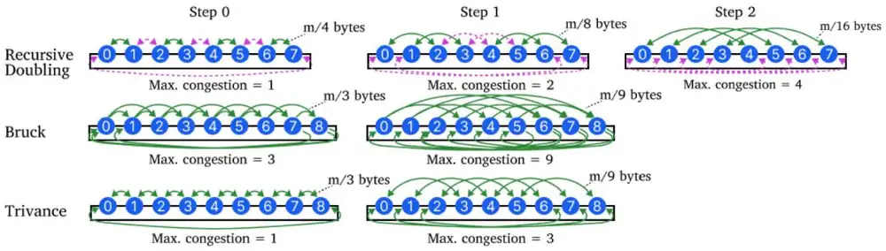
The table restates the figure (all values are counts from the schedules, not measurements):

下表重述這張圖（數值都是由排程數出來的，不是量測）：

Schedule (ring size)排程（環的大小）	Steps步數	Use of the second port第二個埠的用法	Link load鏈路負載
Recursive doubling (8)遞迴倍增（8）	3	independent mirrored copy獨立的 mirrored 副本	at most 1, 2, then 4 messages per link每條鏈路最多 1、2、4 則訊息
Bruck (9)Bruck（9）	2	second message, same direction第二則訊息，同一方向	at most 3, then 9; all traffic one way, reverse links idle最多 3、9 則；全部流量走同一方向，反向鏈路閒置
Trivance (9)Trivance（9）	2	second peer, opposite direction第二個夥伴，反方向	exactly 1, then 3, on every link每條鏈路恰好 1、3 則

The paper's motivation is cited, not measured: on large production systems more than 40% of MPI time goes to all-reduce and reduce, and TPU v4 builds 3D tori of up to 4,096 chips.

論文的動機是引用而非自己量測：在大型正式系統上，超過 40% 的 MPI 時間花在 all-reduce 與 reduce，而 TPU v4 以最多 4,096 顆晶片組成三維環面。

3. The design3. 設計

3.1 Two peers per step, reduced together3.1 每步兩個夥伴，一起歸約

In step $k$ , node $r$ of an $n$ -node ring talks to two peers at once:

在 $n$ 個節點的環上，第 $k$ 步節點 $r$ 同時與兩個夥伴通訊：

\begin{aligned} \pi_{\text{left}} &= r - 3^k \bmod n \\ \pi_{\text{right}} &= r + 3^k \bmod n \end{aligned}

It must receive and reduce both inputs, with its own partial result, before it sends in step $k+1$ . The paper calls this joint reduction. By Lemma 4.2, after step $k$ node $r$ holds the data of every node within distance

它必須收到兩個輸入，並與自己的部分結果一起歸約，才能在第 $k+1$ 步送出。論文稱之為聯合歸約（joint reduction）。依 Lemma 4.2，第 $k$ 步之後，節點 $r$ 持有距離在下列範圍內所有節點的資料：

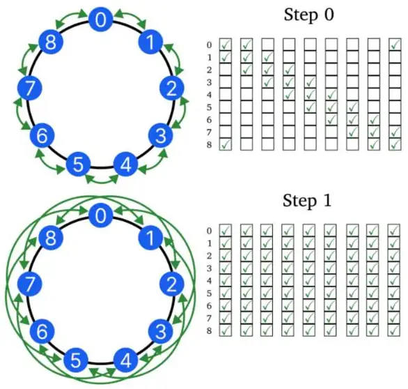
R_k = \sum_{i=0}^{k} 3^i = \frac{3^{k+1} - 1}{2} \qquad (1,\ 4,\ 13,\ 40,\ \dots)

Why (Appendix A): the $3^{k+1} - 1$ nodes between $r$ and its right peer split into two ranges of $R_k$ nodes, one known to $r$ and one known to the peer. Each exchange brings only new data, so the covered set triples each step (Figure 1). For $n = 3^s$ the ring's diameter equals $R_{s-1}$ , so $s$ steps reach every node.

原因（附錄 A）： $r$ 與右側夥伴之間的 $3^{k+1} - 1$ 個節點分成兩段，各 $R_k$ 個，一段 $r$ 已知，另一段夥伴已知。每次交換帶來的都是新資料，所以涵蓋的集合每步變三倍（圖 1）。當 $n = 3^s$ ，環的直徑等於 $R_{s-1}$ ，所以 $s$ 步就能到達每個節點。

Figure 1. The nodes whose data rank

r

(outlined) holds after each step, on 27 positions around

r

. Solid cells are new in that step, half-transparent cells were known before, and dots mark that step's peers. Swing's set doubles (2, 4, 8); Trivance's triples (3, 9, 27), so 27 nodes need 3 steps instead of 5.圖 1。rank

r

（外框）在每一步之後持有哪些節點的資料，畫出

r

周圍 27 個位置。實心格子是該步新增的，半透明格子是先前已知的，圓點標出該步的夥伴。Swing 的集合每步加倍（2、4、8）；Trivance 的集合每步變三倍（3、9、27），所以 27 個節點只要 3 步而不是 5 步。Drawn for this primer from Lemma 4.2 of Juerss, Addanki and Schmid, SIGCOMM 2026, and Eq. 2 of the Swing paper.

The paper's Figure 3 (below) follows every node on a 9-node ring: node 0 gets nodes 1 and 8 in step 0, then 2, 3 and 4 through node 3, and 5, 6 and 7 through node 6.

論文的 Figure 3（下圖）追蹤 9 節點環上的每個節點：節點 0 在第 0 步得到節點 1 與 8 的資料，接著經由節點 3 得到 2、3、4，經由節點 6 得到 5、6、7。

Two ring diagrams of nine nodes with exchange arrows, each beside a 9 by 9 grid of ticks showing which blocks each node holds. — Figure 3 of the paper: received blocks on a 9-node ring (an algorithm schematic). In each grid, column $c$ lists the nodes whose data node $c$ holds. After step 0 every column has 3 ticks (itself and both neighbours); after step 1, through the peers 3 hops away, it has all 9 — the count triples each step, so $\lceil \log_3 n \rceil$ steps are enough.論文圖 3：9 節點環上收到的區塊（演算法示意圖）。每個網格中，第 $c$ 欄列出節點 $c$ 持有哪些節點的資料。第 0 步後每欄有 3 個勾（自己與兩個鄰居）；第 1 步經由相隔 3 跳的夥伴後就有全部 9 個——數量每步變三倍，所以 $\lceil \log_3 n \rceil$ 步就夠。Juerss, Addanki and Schmid, SIGCOMM 2026, Figure 3 (camera-ready PDF, p. 7, re-rendered).

3.2 Bandwidth-optimal form and the congestion bill3.2 頻寬最佳的形式與壅塞的帳單

The bandwidth-optimal form splits the vector into $n$ blocks and runs a reduce-scatter, then an all-gather. In step $k$ , node $r$ sends each peer the blocks for that peer and for every node the peer reaches later: $3^{s-1-k}$ blocks, or $m/3^{k+1}$ bytes, where $s = \log_3 n$ . Lemma 4.1 sums both peers over one phase:

頻寬最佳的形式把向量切成 $n$ 個區塊，先跑 reduce-scatter，再跑 all-gather。第 $k$ 步，節點 $r$ 送給每個夥伴的是該夥伴、以及該夥伴之後會到達的每個節點的區塊：共 $3^{s-1-k}$ 個區塊，即 $m/3^{k+1}$ 位元組，其中 $s = \log_3 n$ 。Lemma 4.1 把兩個夥伴在一個階段內的量加總：

\sum_{k=0}^{s-1} 2 \cdot \frac{m}{3^{k+1}} = m\left(1 - 3^{-s}\right) = m\left(1 - \frac{1}{n}\right)

So the two phases send the minimal $2m(1 - 1/n)$ bytes in $2\lceil \log_3 n \rceil$ steps. The cost model charges each step $\alpha$ plus $\beta m_k c_k$ , with $c_k$ the chunks that share a link. Both peers sit $3^k$ hops away, so every link carries exactly $3^k$ chunks. The payload falls by 3 as the load rises by 3, so the byte factor $\Theta$ (in units of $m\beta$ ) is $\tfrac23 \log_3 n$ . Bruck's messages travel $3^k$ and $2 \cdot 3^k$ hops the same way, so its links carry three times as many chunks. The paper's Table 1 (model values):

所以兩個階段以 $2\lceil \log_3 n \rceil$ 步送出最少的 $2m(1 - 1/n)$ 位元組。成本模型對每一步收 $\alpha$ 加上 $\beta m_k c_k$ ， $c_k$ 是共用一條鏈路的 chunk 數。兩個夥伴都隔 $3^k$ 跳，所以每條鏈路恰好承載 $3^k$ 個 chunk。酬載除以 3、負載乘以 3，所以位元組因子 $\Theta$ （以 $m\beta$ 為單位）是 $\tfrac23 \log_3 n$ 。Bruck 的兩則訊息往同一方向走 $3^k$ 與 $2 \cdot 3^k$ 跳，所以它的鏈路承載三倍的 chunk。論文的 Table 1（模型值）：

Ring, two ports環，兩個埠	Steps (B)步數 (B)	$\Theta$ (B)	Steps (L)步數 (L)	$\Theta$ (L)
Ring環	$2(n-1)$	$1$	—	—
Recursive doubling遞迴倍增	$2\log_2 n$	$\tfrac12 \log_2 n$	$\log_2 n$	$n$
Swing	$2\log_2 n$	$\tfrac13 \log_2 n$	$\log_2 n$	$n/3$
Bruck	$2\lceil \log_3 n \rceil$	$2\log_3 n$	$\lceil \log_3 n \rceil$	$3n/2$
Trivance	$2\lceil \log_3 n \rceil$	$\tfrac23 \log_3 n$	$\lceil \log_3 n \rceil$	$n/2$

(B) is the bandwidth-optimal form; (L), the latency-optimal form, forwards the whole vector in every step. The (L) columns show the trade-off: Trivance saves steps but puts 1.5 times Swing's byte load on the busiest links, so the winner depends on $\alpha$ against $\beta m$ .

(B) 是頻寬最佳的形式；(L) 是延遲最佳的形式，每一步都轉送整個向量。(L) 欄呈現了取捨：Trivance 省下步數，但在最忙的鏈路上放了 Swing 1.5 倍的位元組負載，所以誰勝出取決於 $\alpha$ 與 $\beta m$ 的大小。

3.3 Sizes that are not a power of three3.3 不是 3 的冪的大小

For other $n$ , Trivance runs $\lfloor \log_3 n \rfloor$ normal steps. In the last step both peers sit at distance $\lceil (n - 3^{\lfloor \log_3 n \rfloor})/2 \rceil$ , just enough to cover the missing nodes. A 32-node ring knows 27 nodes before its last step and needs 5 more, while an 81-node ring would need 54. The step count stays $\lceil \log_3 n \rceil$ . Figure 2 shows the paper's Table 2.

對其他的 $n$ ，Trivance 先跑 $\lfloor \log_3 n \rfloor$ 個一般步驟。最後一步兩個夥伴的距離是 $\lceil (n - 3^{\lfloor \log_3 n \rfloor})/2 \rceil$ ，剛好補齊缺少的節點。32 節點的環在最後一步前已知 27 個節點，只需再補 5 個；81 節點的環則需要 54 個。步數仍是 $\lceil \log_3 n \rceil$ 。圖 2 呈現論文的 Table 2。

Figure 2. Peer distance in each step of Trivance for four ring sizes; the last step (orange) is shortened. Right: the last step's congestion relative to the last step of the next power of three. A 32-node ring pays 11% of an 81-node ring's last step, a 64-node ring 70%.圖 2。四種環大小下 Trivance 每一步的夥伴距離；最後一步（橘色）被縮短。右：最後一步的壅塞，相對於下一個 3 的冪的最後一步。32 節點的環只付出 81 節點環最後一步的 11%，64 節點的環則是 70%。Drawn for this primer from §4.4 and Table 2 of Juerss, Addanki and Schmid, SIGCOMM 2026 (model values).

Against $\lceil \log_2 n \rceil$ , the paper counts 25–57% more steps for Swing and recursive doubling at power-of-two sizes, up to 75% at other sizes, and 58.5% as $n$ grows ( $\log_2 3 \approx 1.585$ ).

與 $\lceil \log_2 n \rceil$ 相比，論文算出：在 2 的冪的大小上，Swing 與遞迴倍增多出 25–57% 的步數，其他大小最多多出 75%， $n$ 變大時多出 58.5%（ $\log_2 3 \approx 1.585$ ）。

3.4 Multidimensional tori3.4 多維環面

On a torus, Trivance runs one collective per dimension, each on $1/D$ of the vector, mapped to distinct dimensions in every step; on a 9×9 torus the two collectives swap dimensions after each step. Messages get smaller and shorter. Table 3 gives the byte factor relative to the optimum $m\beta/D$ ; for Trivance (B) it is $(3^D - 1)/(3^D - 3)$ (Figure 3).

在環面上，Trivance 每個維度跑一個集體操作，各處理向量的 $1/D$ ，每一步對應到不同的維度；在 9×9 環面上，兩個集體操作每一步都互換維度。訊息變小、距離變短。Table 3 給出相對最佳值 $m\beta/D$ 的位元組因子；Trivance (B) 是 $(3^D - 1)/(3^D - 3)$ （圖 3）。

Figure 3. Byte factors of the bandwidth-optimal forms on 2D, 3D and 4D tori (Table 3, model values for large

n

), drawn as the excess over the optimum on a log scale. The bucket algorithm is exactly optimal. In 3D and 4D Trivance is within 8% and 2%, while it keeps its smaller step count.圖 3。頻寬最佳形式在 2D、3D、4D 環面上的位元組因子（Table 3，

n

很大時的模型值），以對數刻度畫出高於最佳值的部分。bucket 演算法恰好最佳。在 3D 與 4D，Trivance 分別只高出 8% 與 2%，同時保有較少的步數。Drawn for this primer from §5 and Table 3 of Juerss, Addanki and Schmid, SIGCOMM 2026.

Panel 1 evaluates the model of Tables 1 and 3 for every ring or torus size and vector size.

面板 1 依 Table 1 與 Table 3 的模型，計算每一種環或環面大小與向量大小。

Panel 1面板 1

Fewer steps or less link load: who wins where, by the paper's model步數較少還是鏈路負載較輕：依論文的模型，誰在哪裡勝出

Topology拓樸

Size (row)大小（列）

Vector size

m

(column)向量大小

m

（欄）

Per-step latency

\alpha

每步延遲

\alpha

Link rate鏈路速率

Steps, Trivance : Swing

步數，Trivance : Swing

\Theta

(L), Trivance : Swing

\Theta

(L)，Trivance : Swing

Fastest at the outlined cell

框起格子中最快

Trivance fastest in this row up to

本列中 Trivance 最快直到

Model values only; the paper's simulated results are not shown. Each cell takes the smallest $T = K\alpha + \Theta\, m\beta/D$ over nine algorithms: $K$ is the step count and $\Theta$ the byte factor of Table 1 (rings, $D = 1$ ) or the large- $n$ forms of Table 3 (tori), with rounded-up logarithms for the steps. Solid cells are latency-optimal forms (L), half-transparent cells bandwidth-optimal ones (B). Bruck and recursive doubling never win in this model: they take as many steps as Trivance and Swing but have a larger $\Theta$ . Defaults: a 64-node ring with the paper's $\alpha = 1.5$ µs and 800 Gb/s links; the model switches from Trivance (L) to (B) at about 20 KiB, to Swing (B) at about 1.1 MiB and to the ring at about 16 MiB. Raise $\alpha$ or the link rate: Trivance's region grows, because each saved step is worth more bytes. Switch to 3D: the byte factors approach 1, so the step count decides more cells. Compare neighboring rows such as 27 and 32: step counts change in jumps, so the regions do too. Table 3's forms are limits for large $n$ , so small tori are rough.

只有模型值；不顯示論文的模擬結果。每個格子從九種演算法中取最小的 $T = K\alpha + \Theta\, m\beta/D$ ： $K$ 是步數， $\Theta$ 是 Table 1（環， $D = 1$ ）或 Table 3 大 $n$ 形式（環面）的位元組因子，步數的對數取上整數。實心格子是延遲最佳形式（L），半透明格子是頻寬最佳形式（B）。在這個模型中 Bruck 與遞迴倍增永遠不會勝出：它們的步數與 Trivance、Swing 相同，但 $\Theta$ 較大。預設值：64 節點的環、論文的 $\alpha = 1.5$ µs 與 800 Gb/s 鏈路；模型約在 20 KiB 從 Trivance (L) 切到 (B)，約 1.1 MiB 切到 Swing (B)，約 16 MiB 切到環。提高 $\alpha$ 或鏈路速率：Trivance 的區域變大，因為每省下一步就相當於更多位元組。切到 3D：位元組因子趨近 1，所以更多格子由步數決定。比較相鄰的列，例如 27 與 32：步數是跳躍式變化，區域也跟著跳。Table 3 的形式是大 $n$ 時的極限，所以小環面只是粗估。

4. Implementation4. 實作

The authors implemented Trivance and Bruck in SST, a packet-level simulator, and took bucket, recursive doubling and Swing from Swing's public code, with recursive doubling extended to all ports. For a fair baseline they improved Bruck: shortest-path routing, joint reductions, and a reversed all-gather after NCCL's PAT algorithm. There is no implementation in a production library.

作者在封包層級模擬器 SST 中實作了 Trivance 與 Bruck，bucket、遞迴倍增與 Swing 則取自 Swing 公開的程式碼，並把遞迴倍增擴充為使用所有的埠。為了公平比較，他們改良了 Bruck：最短路徑繞送、聯合歸約，以及仿照 NCCL PAT 演算法的反向 all-gather。沒有在正式函式庫中的實作。

Appendix D (not peer-reviewed) sketches one: a backend schedule like PAT emits one work item per rank, step and chunk, with both peers, and a per-chunk readiness entry with two bits lets the reduction run only when both receives are done (Figure 4). A library should pick Trivance only if each dimension has two independent paths.

附錄 D（未經同儕審查）勾勒了一種實作：後端排程像 PAT 一樣，為每個 rank、步驟與 chunk 產生一個帶有兩個夥伴的工作項目，而每個 chunk 的就緒項目有兩個位元，兩個接收都完成後才執行歸約（圖 4）。函式庫應該只在每一維都有兩條獨立路徑時才選用 Trivance。

Figure 4. One chunk in a PAT step and in a Trivance step. Trivance's reduction waits for two receives, so a late input stalls the pair.圖 4。同一個 chunk 在 PAT 的一步與 Trivance 的一步中的流程。Trivance 的歸約要等兩個接收完成，所以一個輸入遲到就會拖住一對。Drawn for this primer from §7 and Appendix D of Juerss, Addanki and Schmid, SIGCOMM 2026.

5. What was evaluated5. 評估了什麼

The simulated network has 800 Gb/s links, 100 ns propagation, about 200 ns per hop, 8,192 B packets, a per-step latency $\alpha = 1.5\,\mu\text{s}$ , $2D$ network interfaces per node with their own engines, credit-based flow control and shortest-path routing. The shapes are rings of 8 and 64 nodes, 2D tori 32×32, 8×64 and 27×27, and a 16×16×16 torus. Link rates range from 200 Gb/s to 3.2 Tb/s, and vectors from 32 B to 128 MiB. The baselines are bucket, recursive doubling, Swing and the improved Bruck, each in its better form. All of the paper's speedups and crossover sizes come from this simulation, so this page does not show them.

模擬的網路使用 800 Gb/s 鏈路、100 ns 傳播延遲、每跳約 200 ns、8,192 B 封包、每步延遲 $\alpha = 1.5\,\mu\text{s}$ ，每節點 $2D$ 個各有獨立引擎的網路介面，以及 credit-based 流量控制與最短路徑繞送。拓樸包括 8 與 64 節點的環、32×32、8×64、27×27 的二維環面，以及 16×16×16 的環面。鏈路速率從 200 Gb/s 到 3.2 Tb/s，向量從 32 B 到 128 MiB。比較基準是 bucket、遞迴倍增、Swing 與改良的 Bruck，各取較好的形式。論文所有的加速倍數與交叉點大小都來自這個模擬，所以本頁不列出。

The model alone gives crossovers. With Table 1, $\alpha = 1.5\,\mu\text{s}$ and 800 Gb/s (100 GB/s) on a 64-node ring, one row per switch (our computation):

只靠模型也能算出交叉點。用 Table 1、 $\alpha = 1.5\,\mu\text{s}$ 與 800 Gb/s（100 GB/s），在 64 節點的環上，每列一個切換點（我們的計算）：

Switch (64-node ring, model)切換（64 節點的環，模型）	Calculation算式	Result結果
Trivance (L) → (B): 4 more steps, $\Theta$ 32 → 2.52Trivance (L) → (B)：多 4 步， $\Theta$ 32 → 2.52	$4 \times 1.5\,\mu\text{s} \times 100\,\text{GB/s} \div (32 - 2.52)$	$\approx 20$ KiB
Trivance (B) → Swing (B): 4 more steps, $\Theta$ 2.52 → 2Trivance (B) → Swing (B)：多 4 步， $\Theta$ 2.52 → 2	$4 \times 1.5\,\mu\text{s} \times 100\,\text{GB/s} \div (2.52 - 2)$	$\approx 1.1$ MiB
Swing (B) → ring: 114 more steps, $\Theta$ 2 → 1Swing (B) → 環：多 114 步， $\Theta$ 2 → 1	$114 \times 1.5\,\mu\text{s} \times 100\,\text{GB/s} \div (2 - 1)$	$\approx 16$ MiB

The simulator adds per-hop delay, packets and finite-size effects, so its crossovers differ from these.

模擬器另外包含每跳延遲、封包化與有限大小的效應，所以它的交叉點與這些值不同。

6. Limits and open questions6. 限制與未解的問題

The paper lists its limits (§7): simulation does not replace a library implementation; joint reduction needs stronger synchronization, and if one peer sends chunks in ascending order and the other in descending order, about half a message waits; Clos fabrics are future work; and using all $2D$ ports at once could reach $\lceil \log_{2D+1} n \rceil$ steps only with very specific sizes. A careful reader should add:

論文列出了自己的限制（§7）：模擬無法取代函式庫中的實作；聯合歸約需要更強的同步，若一個夥伴以遞增順序送 chunk、另一個以遞減順序送，大約半個訊息要等待；Clos 網路是未來的工作；同時使用全部 $2D$ 個埠只有在非常特定的大小下才能達到 $\lceil \log_{2D+1} n \rceil$ 步。細心的讀者還應該補上：

Power-of-two sizes are common. At 64 nodes the last step costs 70% of the 81-node case (Figure 2).2 的冪的大小很常見。64 個節點時，最後一步的成本是 81 節點情況的 70%（圖 2）。
Endpoint model. Each simulated interface injects on its own, with no node-wide limit. A GPU whose two streams share one NIC or PCIe path would serialize them.端點模型。每個模擬的介面各自注入，沒有全節點的上限。若 GPU 的兩條資料流共用一張 NIC 或同一條 PCIe 路徑，就會被串行化。
Reduction cost. The model leaves out $\gamma$ , although each step reduces three operands. The paper notes that the reduced volume falls from about $2m$ to $1.5m$ .歸約成本。模型沒有包含 $\gamma$ ，雖然每一步要歸約三個運算元。論文指出歸約的總量從約 $2m$ 降到 $1.5m$ 。
No straggler test, although joint reduction is more sensitive to a late input than independent copies.沒有 straggler 測試，雖然聯合歸約比獨立的副本更怕輸入遲到。

7. How it connects7. 與其他內容的關聯

Swing (NSDI 2024) is the direct predecessor: same simulator, same direct-connect setting, and the strongest baseline. Swing cuts distance; Trivance cuts steps.Swing（NSDI 2024）是直接的前作：相同的模擬器、相同的直連拓樸情境，也是最強的比較基準。Swing 削減距離；Trivance 削減步數。
Deep dive: Panel 4 (section 4) animates Trivance's peers; section 9.2 gives its step table.第 4 章：面板 4（第 4 節）以動畫呈現 Trivance 的夥伴；第 9.2 節給出它的步數表。
TPU v4 is the paper's target: 3D tori of up to 4,096 chips, where the 3D column of Table 3 applies.TPU v4 是論文的目標：最多 4,096 顆晶片的三維環面，正適用 Table 3 的 3D 欄。
Theseus, in the same SIGCOMM session, hot-swaps schedules at run time; a Trivance schedule could be one entry in its menu.Theseus 與本文同屬 SIGCOMM 的同一場議程，能在執行期熱抽換排程；Trivance 的排程可以是它選單中的一項。

Key numbers關鍵數字

Number	數字	Meaning (kind of value)
$\lceil \log_3 n \rceil$	Steps of latency-optimal Trivance; the two-port lower bound (proof)	延遲最佳 Trivance 的步數；兩埠的下限（證明）
≈ 37%	Fewer steps than $\log_2 n$ , as $n$ grows (analysis)	$n$ 變大時比 $\log_2 n$ 少的步數（分析）
$3^k$ · 3×	Chunks per link in step $k$ ; Bruck's load relative to Trivance (analysis)	第 $k$ 步每鏈路的 chunk 數；Bruck 相對 Trivance 的負載（分析）
$n/2$ vs $n/3$	$\Theta$ of latency-optimal Trivance vs Swing (Table 1, model)	延遲最佳 Trivance 與 Swing 的 $\Theta$ （Table 1，模型）
1.33 / 1.08 / 1.02	$\Theta$ of Trivance (B) on 2D / 3D / 4D tori (Table 3, model)	Trivance (B) 在 2D／3D／4D 環面的 $\Theta$ （Table 3，模型）
11.1% · 70.4%	Last-step congestion of 32 and 64 nodes vs 81 (Table 2, model)	32 與 64 節點最後一步相對 81 的壅塞（Table 2，模型）
800 Gb/s · 1.5 µs	Simulated link rate and per-step latency (setup)	模擬的鏈路速率與每步延遲（設定）

Terms used on this page本頁用到的術語

Joint reduction: Reducing both incoming messages of a step with the local partial result before forwarding.; 在轉送前，把一步中收到的兩則訊息與本地部分結果一起歸約。
Bruck's algorithm: A two-port all-gather in $\log_3 n$ steps, with peers at $3^k$ and $2 \cdot 3^k$ in one direction.; 兩個埠下以 $\log_3 n$ 步完成的 all-gather，夥伴在同一方向的 $3^k$ 與 $2 \cdot 3^k$ 。
Byte factor $\Theta$: The sum over steps of bytes sent times chunks per link, relative to $m\beta$ (ring) or $m\beta/D$ (torus).; 各步送出的位元組乘以每鏈路 chunk 數之和，相對於 $m\beta$ （環）或 $m\beta/D$ （環面）。
(L) / (B) form: Latency-optimal: the whole vector in every step. Bandwidth-optimal: reduce-scatter plus all-gather with the minimal bytes.; 延遲最佳：每步送整個向量。頻寬最佳：reduce-scatter 加 all-gather，位元組最少。
PAT: NCCL's Bruck-derived all-gather and reduce-scatter.; NCCL 由 Bruck 衍生的 all-gather 與 reduce-scatter。