Swing: Short-cutting Rings for Higher Bandwidth AllreduceSwing:抄捷徑繞過環,提升 allreduce 頻寬
After reading, you can explain why two all-reduce schedules with equal steps and bytes run at different speeds on a torus, and how Swing's alternating peers cut link sharing.讀完後,你能說明為什麼步數與位元組都相同的兩種 all-reduce 排程,在環面上速度不同,以及 Swing 左右交替的夥伴如何減少鏈路共用。
On a torus, a message to a peer hops away occupies links, so the messages of one collective share links. Recursive doubling and Rabenseifner's algorithm pair rank with , so the distance doubles at every step and the late steps congest. Swing keeps their steps and minimal bytes, but uses the offsets : even ranks add them and odd ranks subtract them, so peers are about two-thirds as far. Plain plus mirrored copies keep all ports busy. The paper's congestion factor is about 1.19, 1.03 and 1.008 on 2D, 3D and 4D tori, against 1.5, 1.17 and 1.07 for Rabenseifner tuned for tori. The evidence is this model plus simulation, so this page teaches the model.
在環面(torus)上,送給 跳外夥伴的訊息會佔用 條鏈路,所以同一集體操作的訊息會共用鏈路。遞迴倍增與 Rabenseifner 演算法把 rank 與 配對,所以距離每步加倍,後面幾步造成壅塞。Swing 保留它們的 步與最少位元組,但改用偏移 :偶數 rank 加上、奇數 rank 減去,所以夥伴只有約三分之二遠。plain 加上 mirrored 副本讓全部 個埠都在工作。論文的壅塞因子 在 2D、3D、4D 環面上約為 1.19、1.03、1.008,針對環面調整的 Rabenseifner 則是 1.5、1.17、1.07。證據是這個模型加上模擬,所以本頁教的是模型。
1. Where this paper sits1. 這篇論文的位置
Section 4.3 builds the – model: each dependent step costs , each byte . There, Rabenseifner's algorithm sends the ring's minimal bytes in only steps, on one condition: every pair of ranks can talk at full rate at once. The primer's Rabenseifner section says why: the later partners sit far apart, so their messages cross more links and share them.
第 4.3 節建立了 – 模型:每個相依步驟花 ,每個位元組花 。在那裡,Rabenseifner 演算法只用 步就送出環的最少位元組,條件是任兩個 rank 能同時以全速通訊。總覽的 Rabenseifner 一節說明原因:後面幾步的夥伴相距很遠,訊息要跨更多鏈路並彼此共用。
A torus breaks that condition, because a message to a distant rank uses other nodes' links. Before Swing, ring and bucket algorithms avoided shared links but needed or about steps; recursive doubling needed steps over long distances; schedule synthesis can take up to 11 hours for 128 nodes (TACCL, cited). Swing changes only the choice of peer. Panel 4 of Chapter 4 (section 4) animates its peers.
環面打破了這個條件,因為送給遠方 rank 的訊息要借用其他節點的鏈路。在 Swing 之前,環與 bucket 演算法避開了共用鏈路,但需要 步或約 步;遞迴倍增只要 步,但距離很長;排程合成在 128 個節點上可能要算 11 小時(TACCL,論文引用)。Swing 只改變夥伴的選法。第 4.4 節的面板 4 以動畫呈現它的夥伴。
2. The problem: same steps, same bytes, different time2. 問題:步數相同、位元組相同,時間卻不同
The paper's Figure 1 (below) makes the point on a 16-node ring (a 1D torus) with shortest-path routing. Both algorithms run the bandwidth-optimal reduce-scatter, so in step each node sends bytes of its -byte vector. In step 1, recursive doubling sends to , two hops away, so two messages cross the links 1–2 and 5–6 in the same direction. Swing sends to the other neighbor, one message per link. In step 2, four doubling messages share the link 3–4; Swing's busiest links carry two.
論文的 Figure 1(下圖)在 16 節點的環(一維環面)上、以最短路徑繞送說明這一點。兩種演算法都執行頻寬最佳的 reduce-scatter,所以第 步每個節點送出 位元組向量中的 。第 1 步,遞迴倍增把 送給兩跳外的 ,所以兩則訊息同向穿過鏈路 1–2 與 5–6。Swing 把 送給另一側的鄰居,每條鏈路一則訊息。第 2 步,遞迴倍增有四則訊息共用鏈路 3–4;Swing 最忙的鏈路只有兩則。
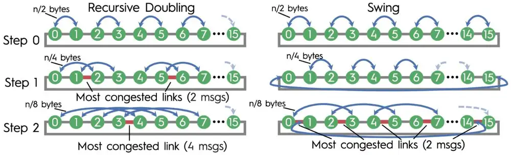
A step lasts as long as its busiest link needs: the payload times the messages that share the link. In units of , the time to send the whole vector over one link:
一步的時間取決於最忙的鏈路:酬載乘以共用該鏈路的訊息數。以 (整個向量走一條鏈路的時間)為單位:
| Step (16-node ring, Figure 1 of the paper)步驟(16 節點的環,論文 Figure 1) | Calculation算式 | Result結果 |
|---|---|---|
| Step 0, both: payload , one message per link第 0 步,兩者:酬載 ,每鏈路一則 | ||
| Step 1: recursive doubling (2 per link) / Swing (1)第 1 步:遞迴倍增(每鏈路 2 則)/Swing(1 則) | ||
| Step 2: recursive doubling (4 per link) / Swing (2)第 2 步:遞迴倍增(每鏈路 4 則)/Swing(2 則) | ||
| Three steps: recursive doubling / Swing三步合計:遞迴倍增/Swing | doubling takes 1.5× as long遞迴倍增要 1.5 倍時間 |
Both send bytes in three steps, yet doubling takes 1.5 times as long, and the – model has no term for this. The paper's motivation is cited, not measured: all-reduce takes up to 40% of training time in other studies, and tori connect ML systems such as TPU v5p pods.
兩者在三步中都送出 位元組,遞迴倍增卻要 1.5 倍時間,而 – 模型沒有描述這件事的項。論文的動機是引用而非自己量測:其他研究指出 all-reduce 最多佔訓練時間的 40%,而環面也連接著 TPU v5p pod 這類 ML 系統。
3. The design3. 設計
3.1 Peers that swing left and right3.1 左右擺盪的夥伴
In step (counted from 0), node of a -node ring exchanges with
在 個節點的環上,第 步(從 0 起算)節點 與下列節點交換:
So runs : even ranks add it and odd ranks subtract it, so the two members of a pair name each other. The hop distance is
所以 依序是 :偶數 rank 加上它、奇數 rank 減去它,所以一對節點會互相指向對方。跳數距離是
It is strictly below doubling's for , and the ratio approaches . Diagram A draws the peers for six steps: Swing reaches far nodes by a shortcut across the ring instead of walking one way.
當 時它嚴格小於遞迴倍增的 ,比值趨近 。示意圖 A 畫出六步的夥伴:Swing 從環的兩側抄捷徑抵達遠處的節點,而不是一路往同一邊走。
Appendix A proves that no block is reduced twice: a node reached through several steps sits at a sum of distinct powers of , and no number has two such representations.
附錄 A 證明沒有區塊會被歸約兩次:經由多步到達的節點位於一組相異的 次方之和,而沒有任何數有兩種這樣的表示法。
3.2 Halve the data, then double it back3.2 先把資料減半,再加倍送回
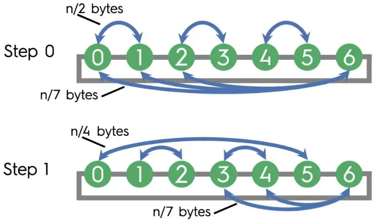
The bandwidth-optimal form is a reduce-scatter, then an all-gather. Each node splits its vector into blocks. In step , node sends its peer the block that will own, plus every block that forwards later (the paper's Listing 1 finds this set recursively), so the payload halves at every step. The all-gather replays the peers in reverse order, farthest first. That is steps () and the minimal bytes (). The latency-optimal form exchanges the whole vector in every step: steps and bytes. For an even that is not a power of two, nodes never send a block twice, at no extra cost. For an odd , nodes run Swing and the last node trades blocks directly, which adds to . The paper's Figure 3 shows .
頻寬最佳的形式先跑 reduce-scatter,再跑 all-gather。每個節點把向量切成 個區塊。第 步,節點 送給夥伴 的是 將負責的區塊,加上 之後要轉交的所有區塊(論文的 Listing 1 以遞迴找出這個集合),所以酬載每步減半。all-gather 以相反順序重走這些夥伴,最遠的先走。合計 步(),位元組為最少的 ()。延遲最佳的形式每步交換整個向量: 步、 位元組。若 是偶數但不是 2 的冪,節點從不重複送同一區塊,不增加成本。若 是奇數,由 個節點跑 Swing,最後一個節點直接交換區塊,讓 增加 。論文的 Figure 3 呈現 的情形。
3.3 All ports, every dimension3.3 所有的埠、每一個維度
On a -dimensional torus, step uses dimension and applies the ring rule to that coordinate, at in-dimension step . To fill all ports, Swing splits the vector into parts. The plain collectives start in different dimensions, and the mirrored ones use the opposite sign. The paper's Figure 4 shows step 0 on a 4×4 torus: node 0 exchanges with nodes 1 and 4 (plain) and with 3 and 12 (mirrored).
在 維環面上,第 步使用第 維,並在該維座標上套用環的規則,維內步數為 。為了用滿 個埠,Swing 把向量切成 份。 個 plain 集體操作從不同維度開始, 個 mirrored 集體操作使用相反的正負號。論文的 Figure 4 呈現 4×4 環面的第 0 步:節點 0 與節點 1、4 交換(plain),並與 3、12 交換(mirrored)。
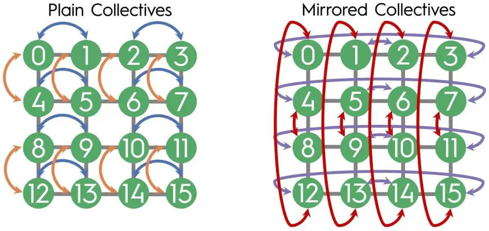
In the next step each collective moves to its other dimension, so the four again use four different ports (Diagram B). So , and the step count does not change.
下一步每個集體操作換到另一個維度,所以四個集體操作仍使用四個不同的埠(示意圖 B)。所以 ,步數不變。
Rectangular tori cost more. After steps the shortest dimension is done, and only two ports carry data. The paper's Eq. 3 approximates the extra congestion as
長方形環面成本較高。經過 步後最短的維度就做完了,之後只有兩個埠載資料。論文的 Eq. 3 把額外的壅塞近似為
For 1,024 nodes that is about 0.021 for 64×16, 0.083 for 128×8 and 0.25 for 256×4 (our evaluation). The paper's Figure 5 shows a 2×4 torus whose last step uses only the horizontal dimension.
對 1,024 個節點,64×16 約 0.021、128×8 約 0.083、256×4 約 0.25(我們代入計算)。論文的 Figure 5 呈現一個 2×4 環面,它的最後一步只用水平維度。
3.4 The congestion factor 3.4 壅塞因子
The paper writes the all-reduce time on a torus with nodes and ports per node as
論文把 個節點、每節點 個埠的環面上 all-reduce 的時間寫成
Here and are the optimum. counts extra steps, extra bytes or idle ports, and the congestion deficiency the slowdown from shared links; only depends on the network. In bandwidth-optimal Swing, step sends bytes per port over hops, so with both phases
其中 與 是最佳值。 計入多出的步數, 計入多出的位元組或閒置的埠,壅塞因子(congestion deficiency) 則是共用鏈路造成的減速;只有 取決於網路。在頻寬最佳的 Swing 中,第 步每個埠送出 位元組、走 跳,所以兩個階段合計
The payload halves at every step, so the long steps carry little data, and the first steps are one hop each. More dimensions therefore put more bytes on one-hop steps (Diagram C).
酬載每步減半,所以長距離的步驟只載很少資料,而前 步每步只走一跳。所以維度越多,走一跳的位元組就越多(示意圖 C)。
The paper's Table 2, bandwidth-optimal rows (model values):
論文 Table 2 的頻寬最佳各列(模型值):
| Algorithm演算法 | on 2D / 3D / 4D:2D / 3D / 4D | ||
|---|---|---|---|
| Hamiltonian rings (2D only)Hamiltonian 環(只限 2D) | 1 | 1 | |
| Bucket | 1 | 1 | |
| Rabenseifner, torus-optimized (one port)Rabenseifner,環面最佳化(單一埠) | 2 | 1.5 / 1.17 / 1.07 | |
| Swing, bandwidth-optimalSwing,頻寬最佳 | 2 | 1 | 1.19 / 1.03 / 1.008 |
For very large vectors only the byte term matters. On a 64×64 torus () the model therefore caps Swing at of peak goodput (our computation). Bucket has but about steps, so it wins only for large vectors. Panel 1 evaluates the whole model.
向量非常大時只剩位元組項重要。所以在 64×64 環面上(),模型把 Swing 的上限定在峰值有效吞吐的 (我們的計算)。bucket 的 ,但約有 步,所以只在向量很大時勝出。面板 1 計算整個模型。
4. Implementation4. 實作
The authors implemented every algorithm in the Structural Simulation Toolkit (SST), a packet-level network simulator: Hamiltonian rings, bucket, both forms of recursive doubling, a mirrored recursive doubling that uses all ports, and both forms of Swing. The paper has no MPI or NCCL implementation and no hardware run. Its SST code is public, and the Trivance paper reuses it.
作者在 Structural Simulation Toolkit(SST,封包層級的網路模擬器)中實作了每一種演算法:Hamiltonian 環、bucket、兩種形式的遞迴倍增、使用所有埠的 mirrored 遞迴倍增,以及兩種形式的 Swing。論文沒有 MPI 或 NCCL 的實作,也沒有在硬體上執行。它的 SST 程式碼是公開的,Trivance 論文就重用了它。
5. What was evaluated5. 評估了什麼
The simulated network has 400 Gb/s links, 100 ns link latency, 300 ns of processing per hop and minimal adaptive routing. The shapes are square 2D tori from 64 to 16,384 nodes, three 1,024-node rectangles (64×16, 128×8, 256×4), 3D and 4D tori, two HammingMesh variants and a HyperX, with link rates from 100 Gb/s to 3.2 Tb/s and vectors from 32 B to 512 MiB or 2 GiB. The baselines are Hamiltonian rings, bucket and recursive doubling. The metric is goodput, vector bytes reduced per second, with a peak of × 400 Gb/s. All of the paper's speedups and crossover sizes come from this simulation, so this page does not show them. The analysis alone gives three results:
模擬的網路使用 400 Gb/s 鏈路、100 ns 鏈路延遲、每跳 300 ns 的處理時間與最小自適應繞送。拓樸包括 64 到 16,384 個節點的正方形二維環面、三種 1,024 節點的長方形(64×16、128×8、256×4)、3D 與 4D 環面、兩種 HammingMesh 與一個 HyperX;鏈路速率從 100 Gb/s 到 3.2 Tb/s,向量從 32 B 到 512 MiB 或 2 GiB。比較基準是 Hamiltonian 環、bucket 與遞迴倍增。指標是有效吞吐(goodput),即每秒歸約的向量位元組數,峰值為 × 400 Gb/s。論文所有的加速倍數與交叉點大小都來自這個模擬,所以本頁不列出。只靠分析就能得到三個結果:
- HyperX links each node to its whole row and column. Swing talks only within a row or column, so every peer is one hop away and .HyperX 讓每個節點連到整列與整行。Swing 只在同列或同行內通訊,所以每個夥伴都只隔一跳,。
- On a non-blocking fat tree neither Swing nor recursive doubling has a congestion term, so the paper expects equal performance.在非阻塞 fat tree 上,Swing 與遞迴倍增都沒有壅塞項,所以論文預期兩者表現相同。
- Mirrored recursive doubling uses all ports like Swing, but its distances stay , so its stays higher.Mirrored 遞迴倍增像 Swing 一樣使用所有的埠,但距離仍是 ,所以 仍然較高。
6. Limits and open questions6. 限制與未解的問題
The paper says that bucket and ring stay better for very large vectors on 2D and elongated tori, that only minimal adaptive routing was tested, and that the model leaves out the reduction cost and the latency that distance adds. A careful reader should add:
論文指出:在二維與細長的環面上,向量非常大時 bucket 與環仍然較好;只測試了最小自適應繞送;模型沒有包含歸約成本 ,也沒有包含距離帶來的延遲。細心的讀者還應該補上:
- No real implementation. There is no MPI or NCCL code and no GPU kernel, although in practice is mostly software and kernel launches.沒有真正的實作。沒有 MPI 或 NCCL 程式碼,也沒有 GPU kernel,而實務上 主要來自軟體與 kernel 啟動。
- Whole slices. The job must own a whole torus with ranks in order: true for a full TPU slice, not for a fragmented allocation.完整的切片。任務必須擁有整個環面且 rank 依序排列:完整的 TPU 切片成立,零碎的配置則不成立。
- Clos fabrics. On the Clos and rail fabrics of most GPU clusters, any two GPUs are a few switch hops apart, so distance is a weak lever.Clos 網路。多數 GPU 叢集使用 Clos 或 rail 網路,任兩顆 GPU 只隔幾跳交換器,所以距離這個槓桿很弱。
- Two normalizations. The Trivance paper re-derives these factors relative to ; read each paper's table in its own model.兩套正規化。Trivance 論文以 為基準重新推導這些因子;每篇論文的表都要在它自己的模型中解讀。
7. How it connects7. 與其他內容的關聯
- Deep dive: Swing adds link sharing to the – model of section 2; Panel 4 (section 4) animates its peers; section 9.2 compares it with Trivance.第 4 章:Swing 在第 2 節的 – 模型中加入鏈路共用;面板 4(第 4 節)以動畫呈現它的夥伴;第 9.2 節把它與 Trivance 比較。
- Trivance (SIGCOMM 2026) is the sequel: it reuses Swing's simulator, sends in both directions in every step and needs only steps.Trivance(SIGCOMM 2026)是續作:它重用 Swing 的模擬器,每一步同時往兩個方向送,只需要 步。
- TPU v4 builds 3D tori of up to 4,096 chips, the shape class of Table 2's 3D column. Rail-only and Alibaba HPN are Clos designs, where Swing's lever is weak.TPU v4 以最多 4,096 顆晶片組成三維環面,正是 Table 2 中 3D 欄的形狀。Rail-only 與 Alibaba HPN 是 Clos 設計,Swing 在那裡的槓桿很弱。
- Theseus swaps schedules while a job runs; Swing could be one more schedule in its menu.Theseus 在任務執行中更換排程;Swing 可以是它選單中多一個排程。
Key numbers關鍵數字
| Number | 數字 | Meaning (kind of value) | 意義(數值類型) |
|---|---|---|---|
| 1, −1, 3, −5, 11 | Swing offsets , steps 0–4 (formula) | Swing 第 0–4 步的偏移 (公式) | |
| ≈ 2/3 | Late peer distance relative to doubling's (analysis) | 後段夥伴距離相對倍增 的比例(分析) | |
| 1.19 / 1.03 / 1.008 | of Swing on 2D / 3D / 4D tori (Table 2, model) | Swing 在 2D/3D/4D 環面的 (Table 2,模型) | |
| 1.5 / 1.17 / 1.07 | of torus-optimized Rabenseifner (Table 2, model) | 環面最佳化 Rabenseifner 的 (Table 2,模型) | |
| 1.184 → 84% | on 64×64 and the goodput ceiling (our computation) | 64×64 的 與有效吞吐上限 (我們的計算) | |
| 400 Gb/s · 300 ns | Simulated link rate and per-hop processing (setup) | 模擬的鏈路速率與每跳處理時間(設定) |
Terms used on this page本頁用到的術語
- Congestion deficiency
- How much the byte term grows because messages of one collective share the busiest link.
- 同一集體操作的訊息共用最忙鏈路,使位元組項變大的倍數。
- ,
- Steps relative to ; bytes or idle ports relative to over ports.
- 步數相對 的倍數;位元組或閒置埠相對於 個埠送 的倍數。
- Plain / mirrored collective
- Swing's concurrent sub-all-reduces, which use a different port in every step.
- Swing 同時執行的 個子 all-reduce,每一步各用不同的埠。
- Bucket algorithm
- Ring reduce-scatter and all-gather along each dimension in turn.
- 沿各維度輪流做環形 reduce-scatter 與 all-gather。
- Goodput
- Vector bytes reduced per second; its all-reduce peak is × link rate.
- 每秒歸約的向量位元組數;all-reduce 的峰值是 × 鏈路速率。