Research digest 1 of 16 · Chapter 4: Collective communication

研究導讀 1 / 16 · 第 4 章：集體通訊

Rethinking Machine Learning Collective Communication as a Multi-Commodity Flow Problem把機器學習的集體通訊重新看成多商品流問題

SIGCOMM 2024Xuting Liu, Behnaz Arzani, Siva Kesava Reddy Kakarla et al. (University of Pennsylvania, Microsoft Research, University of Washington, OpenAI) · paper論文

After reading, you can explain how TE-CCL writes a GPU collective as a multi-commodity flow on a time-expanded graph, why copy forces integer variables, and what hours of solver time buy on real GPUs.讀完後，你能說明 TE-CCL 如何把 GPU 集體操作寫成時間展開圖上的多商品流、為什麼「複製」逼出整數變數，以及數小時的求解時間在真實 GPU 上換到什麼。

≈ 11 min · 1 interactive panel · 5-question quiz≈ 11 分鐘 · 1 個互動面板 · 5 題測驗Chapter 4 ↗第 4 章 ↗Jump to the quiz ↓跳到測驗 ↓

If you read nothing else

只讀這一段也可以

Exact schedule solvers stall beyond one or two chassis. TE-CCL borrows traffic engineering: it copies the topology once per time slot (an epoch), treats every chunk as a commodity, and adds what WAN traffic engineering lacks: finite transfers, copies at GPUs, per-link latency and buffers. The result is an exact mixed-integer program, an LP that stays exact when no GPU must copy (AllToAll), and a round-by-round solver for scale. On a 32-GPU AMD testbed its AllGather schedules reached 2.14× the algorithm bandwidth of TACCL and 3.18× that of RCCL. Solving took under a second for small cases and up to 7 hours at 128 GPUs.

精確的排程求解器超過一兩台機箱就跑不動。TE-CCL 借用流量工程（traffic engineering）：把拓樸在每個時間槽（epoch）複製一份，把每個 chunk 當成一種商品，並補上 WAN 流量工程所缺的部分：有限的傳輸量、GPU 上的複製、每條鏈路的延遲與緩衝區。結果是一個精確的混合整數規劃、一個在沒有 GPU 需要複製時（AllToAll）仍然精確的 LP，以及一個逐輪求解、用來擴大規模的求解器。在 32 GPU 的 AMD 測試平台上，它的 AllGather 排程達到 TACCL 的 2.14 倍、RCCL 的 3.18 倍演算法頻寬。小案例的求解不到一秒，128 顆 GPU 時最多要 7 小時。

1. Where this paper sits1. 這篇論文的位置

The Chapter 4 prices a collective with the $\alpha$ – $\beta$ model (section 2) and shows that a ring or a tree does not fit a server with fast NVLink and slower NICs (section 4). Section 9.1 introduces schedule synthesis: a solver decides which chunk crosses which link at which time. Before TE-CCL, SCCL was exact but handled only one or two chassis; the SIGCOMM text calls it MSCCL, its new name. TACCL scaled further with a human-written sketch and chose routes before the order of sends. WAN traffic engineering (TE) already solves problems of this size, with known optimality gaps, so the authors write the collective as a TE problem.

第 4 章用 $\alpha$ – $\beta$ 模型為集體操作定價（第 2 節），並說明環或樹不適合 NVLink 很快、NIC 較慢的伺服器（第 4 節）。第 9.1 節介紹排程合成（schedule synthesis）：由求解器決定哪個 chunk 在什麼時間走哪條鏈路。在 TE-CCL 之前，SCCL 是精確的，但只能處理一兩台機箱；SIGCOMM 版本用它的新名字 MSCCL 稱呼它。TACCL 靠人寫的 sketch 擴大規模，先選路由、再排傳送順序。WAN 流量工程（TE）早已解過這種規模的問題，而且最佳性差距已知，所以作者把集體操作寫成 TE 問題。

2. The problem, measured2. 問題，用量測說話

The paper's own measurements here are solver run times. On a DGX-1 topology, SCCL needed more than a day for an AllGather with more than 3 chunks per GPU, and its instance mode gave no AllGather with more than 1 chunk after 3 days. TACCL ran out of memory on the larger internal topologies, crashed when it needed more than 400 GB of RAM, and hit time limits of 2 + 2 or 4 + 4 hours for routing plus scheduling.

論文在這裡自己量的是求解器的執行時間。在 DGX-1 拓樸上，SCCL 對每顆 GPU 超過 3 個 chunk 的 AllGather 需要一天以上，它的 instance 模式在 3 天後仍給不出超過 1 個 chunk 的 AllGather。TACCL 在較大的內部拓樸上記憶體不足，需要超過 400 GB RAM 時當掉，並撞上路由加排程 2 + 2 或 4 + 4 小時的時間上限。

Classical TE assigns steady rates and conserves flow at every node, so it cannot be reused as it is. Figure 1 shows the four mismatches that the paper names. The paper's toy examples there are analysis, not measurements.

傳統 TE 分配穩定速率，並在每個節點維持流量守恆，所以不能直接拿來用。圖 1 畫出論文列出的四項不符。那裡的玩具範例是分析，不是量測。

Figure 1. Four assumptions of classical TE that a collective breaks (§2.2). ② is the paper's Figure 2a: a 1 MB chunk and links with zero latency and 1 MB/s; ③ and ④ are simplified. All times come from the paper's toy analysis.圖 1。集體操作打破的四項傳統 TE 假設（§2.2）。② 即論文的 Figure 2a：一個 1 MB 的 chunk，鏈路零延遲、1 MB/s；③ 與 ④ 經過簡化。所有時間都來自論文玩具範例的分析。Drawn for this primer from Liu et al., SIGCOMM 2024, §2.2 and Figure 2.

3. The design3. 設計

3.1 Unroll time: the time-expanded graph3.1 把時間攤開：時間展開圖

TE-CCL cuts time into epochs of length $\tau$ . The time-expanded graph has one copy of every node per epoch. A link $(i,j)$ becomes edges from $(i,k)$ to $(j,\,k+1+\lceil X_{ij}\rceil)$ , where $X_{ij} = \alpha_{ij}/\tau$ is the link's latency in epochs. A buffer edge from $(i,k)$ to $(i,k+1)$ lets a GPU hold data. Switches have no buffer edges, and crossing one costs two link latencies. Each chunk $c$ of source $s$ is a commodity; the demand $D(s,d,c)$ is 1 if destination $d$ wants it. (The paper writes $\alpha$ as $U$ and $\beta$ as $V$ .) In Figure 2, two chunks need link W→C, which carries one chunk per epoch, so chunk b waits one epoch in GPU B's buffer.

TE-CCL 把時間切成長度 $\tau$ 的 epoch。時間展開圖（time-expanded graph）在每個 epoch 都有每個節點的一份複本。鏈路 $(i,j)$ 變成從 $(i,k)$ 到 $(j,\,k+1+\lceil X_{ij}\rceil)$ 的邊，其中 $X_{ij} = \alpha_{ij}/\tau$ 是以 epoch 計的鏈路延遲。從 $(i,k)$ 到 $(i,k+1)$ 的緩衝邊讓 GPU 能留住資料。交換器沒有緩衝邊，穿過一台交換器要付兩次鏈路延遲。來源 $s$ 的每個 chunk $c$ 是一種商品（commodity）；若目的地 $d$ 需要它，需求 $D(s,d,c)$ 為 1。（論文把 $\alpha$ 寫成 $U$ 、 $\beta$ 寫成 $V$ 。）在圖 2 中，兩個 chunk 都需要每個 epoch 只承載一個 chunk 的 W→C，所以 chunk b 在 GPU B 的緩衝區多等一個 epoch。

Figure 2. A time-expanded graph drawn from §3.1 and Appendix C, in which each column is the start of epoch

k

, while grey edges are every possible send or hold. The switch W must forward in the next epoch whatever it receives, and W→C is busy with a, so b waits on B's buffer edge.圖 2。依 §3.1 與附錄 C 繪製的時間展開圖，每一欄是 epoch

k

的開始，灰色邊則是所有可能的傳送或持有。交換器 W 收到什麼都必須在下一個 epoch 轉出，而 W→C 正在送 a，所以 b 停在 B 的緩衝邊上等待。Drawn for this primer from Liu et al., SIGCOMM 2024, §3.1 and Appendix C.

Sizing the epoch by the slowest link is simplest, but time becomes coarse: a chunk that crosses a fast link in a fraction of an epoch still waits the whole epoch before it moves on. So most results size the epoch by the fastest link and treat a slow link like latency: one chunk occupies it for several epochs.

用最慢的鏈路決定 epoch 最簡單，但時間會變粗：在快鏈路上只需一小段時間的 chunk，仍要等完整個 epoch 才能繼續。所以多數結果改用最快的鏈路決定 epoch，並把慢鏈路當成延遲：一個 chunk 會佔用它好幾個 epoch。

3.2 The constraints3.2 限制式

$F_{s,i,j,k,c}$ is the amount of chunk $(s,c)$ that link $(i,j)$ carries from the start of epoch $k$ ; $B_{s,i,k,c}$ is what node $i$ holds then; $R_{s,d,k,c}$ is what destination $d$ has read. Four constraints define a valid schedule (§3.1, without the special first and last epochs). First, capacity:

$F_{s,i,j,k,c}$ 是鏈路 $(i,j)$ 從 epoch $k$ 開始時承載的 chunk $(s,c)$ 數量； $B_{s,i,k,c}$ 是節點 $i$ 這時持有的量； $R_{s,d,k,c}$ 是目的地 $d$ 已讀取的量。四條限制式定義合法的排程（§3.1，略去第一個與最後一個 epoch 的特殊處理）。第一，容量：

\sum_{s}\sum_{c} F_{s,i,j,k,c} \;\le\; \mathrm{cap}_{ij}\,\tau

Second, conservation with copy: what a node holds plus what arrives must cover its largest single outgoing send. The maximum, not a sum, is the copy: one chunk may leave on every outgoing link in the same epoch.

第二，允許複製的守恆：節點持有的量加上抵達的量，必須涵蓋它最大的單一外送量。用最大值而不是總和，這就是複製：一個 chunk 可以在同一個 epoch 從每一條外送鏈路離開。

\begin{array}{l} B_{s,i,k,c} + \displaystyle\sum_{j:(j,i)\in E} F_{s,j,i,\,k-\lceil X_{ji}\rceil,\,c} \\ \qquad \ge\; \displaystyle\max_{j:(i,j)\in E} F_{s,i,j,\,k+1,\,c} \end{array}

Third, a GPU keeps everything it receives, which costs nothing in AllGather (Appendix B limits buffers):

第三，GPU 留下收到的一切，這在 AllGather 中沒有代價（附錄 B 有緩衝區受限的版本）：

B_{s,i,k,c} = B_{s,i,k-1,c} + \sum_{j:(j,i)\in E} F_{s,j,i,\,k-\lceil X_{ji}\rceil-1,\,c}

Fourth, a destination may also relay, so its read is capped by its demand, and by the last epoch $K$ every demand is met:

第四，目的地也可以轉送，所以它的讀取量以需求為上限，而且在最後一個 epoch $K$ 之前每個需求都要滿足：

\begin{array}{l} R_{s,d,k,c} = \min\big(D(s,d,c),\; B_{s,d,k+1,c}\big) \\ R_{s,d,K,c} = D(s,d,c) \end{array}

The objective rewards early delivery: a unit read in epoch $k$ scores $1/(k+1)$ .

目標函數獎勵提早送達：在 epoch $k$ 讀到的一單位得分 $1/(k+1)$ 。

\max \sum_{k}\ \sum_{s \ne d} \frac{R_{s,d,k}}{k+1}

A penalty for useless sends slowed the solver, so a post-processing pass deletes every flow that no demand uses, in $O(|V|+|E|)$ time.

懲罰無用傳送的項會拖慢求解器，所以改由一輪後處理刪掉沒有任何需求用到的流量，耗時 $O(|V|+|E|)$ 。

3.3 Why copy forces integers3.3 為什麼複製逼出整數

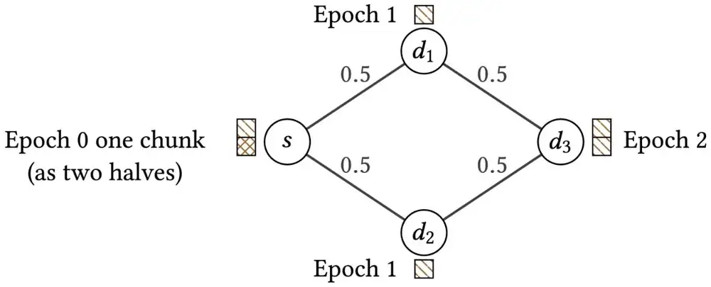
If chunks could be split, the max constraint breaks (the paper's Figure 4, below). Both relays forward the same half to d₃, each forward is legal, and d₃ counts $0.5 + 0.5 = 1$ chunk while it holds one half. Integer chunk variables prevent this. They make the model a mixed-integer linear program (MILP), much slower to solve than an LP of the same size.

如果 chunk 可以切分，最大值限制式就會失效（見下方論文的 Figure 4）。兩個轉送者都把同一半轉給 d₃，每次轉送都合法，而 d₃ 算成收到 $0.5 + 0.5 = 1$ 個 chunk，實際只持有一半。整數的 chunk 變數防止這種情況，也讓模型成為混合整數線性規劃（MILP），比同樣大小的 LP 難解得多。

Figure 4 of the TE-CCL paper: source s, relays d1 and d2, destination d3; links labelled 0.5; the same hatched half reaches d1 and d2 in epoch 1 and arrives twice at d3 in epoch 2. — Figure 4 of the paper (a design example). In epoch 0 the source holds one chunk as two halves and sends the same half (diagonal hatching) to d₁ and d₂; the 0.5 labels are half-chunk flows. In epoch 2, d₃ holds two halves with the same hatching: one half, counted twice. Integer chunk variables rule this out.論文的 Figure 4（設計範例）。epoch 0 時來源把一個 chunk 當成兩半持有，並把同一半（斜線）送給 d₁ 與 d₂；0.5 的標示是半個 chunk 的流量。epoch 2 時 d₃ 持有兩個斜線相同的半塊：其實是同一半被算了兩次。整數的 chunk 變數排除了這種情況。Screenshot of Liu et al., SIGCOMM 2024, Figure 4 (ACM PDF, p. 5).

Panel 1 lets you write a schedule by hand on the paper's Figure 2a topology and check it against these constraints.

面板 1 讓你在論文 Figure 2a 的拓樸上親手寫排程，並用這些限制式檢查它。

Panel 1面板 1

Write a schedule on the time-expanded graph在時間展開圖上寫一份排程

Load a schedule載入排程

Conservation rule守恆規則

Chunks at ss 的 chunk 數

Link latency

\alpha

(one epoch

\tau

= 1 s)鏈路延遲

\alpha

（一個 epoch

\tau

= 1 s）

Demands met

已滿足的需求

Constraint check

限制式檢查

Finish, epoch model

完成時間（epoch 模型）

Same routes, sent when ready

同樣路由，就緒即送

Best here: copy / no copy

此處最佳：複製 / 不複製

Sends that add nothing

沒有貢獻的傳送

Variables in this model

此模型的變數數

Defaults: the paper's Figure 2a. One 1 MB chunk at s must reach d₁, d₂ and d₃ through h; the four links have zero latency and 1 MB/s, so one epoch is $\tau = 1$ s. The default rule is flow conservation ("No copy"), and the loaded schedule sends the chunk three times over s→h: 4 s. Choose "Copy allowed" and load "With copy" for the paper's 2 s. Click a cell to change which chunk a link carries in that epoch. A chunk sent in epoch $k$ can leave the receiver in epoch $k+1+\lceil \alpha/\tau \rceil$ (§3.1). Under "No copy", a unit that reaches h can leave it only once, and s supplies one unit per destination. Dashed cells add nothing (post-processing deletes them); a red cell breaks a constraint. "Sent when ready" runs the same routes, in the same order on each link, but starts each send as soon as its chunk and its link are ready and charges $\alpha + \beta s$ per hop, as a runtime would; it shows slack in your epochs and the cost of rounding $\alpha$ up (try $\alpha = 0.5$ s). The variable count is $F$ (1 source × 4 links × 10 epochs × chunks) plus $B$ (1 source × 5 nodes × 10 epochs × chunks).

預設值：論文的 Figure 2a。s 上一個 1 MB 的 chunk 必須經 h 送到 d₁、d₂ 與 d₃；四條鏈路零延遲、1 MB/s，所以一個 epoch 是 $\tau = 1$ s。預設規則是流量守恆（「不複製」），載入的排程在 s→h 上把 chunk 送三次：4 s。選「允許複製」並載入「有複製」，可得到論文的 2 s。點選格子可以改變某條鏈路在該 epoch 承載哪個 chunk。在 epoch $k$ 送出的 chunk，可以在 epoch $k+1+\lceil \alpha/\tau \rceil$ 從接收端再送出（§3.1）。在「不複製」下，抵達 h 的一單位只能離開一次，而 s 為每個目的地提供一單位。虛線格子沒有貢獻（後處理會刪掉）；紅色格子違反限制式。「就緒即送」使用同樣的路由、每條鏈路上同樣的順序，但每次傳送都在 chunk 與鏈路就緒時立刻開始，每跳收 $\alpha + \beta s$ ，就像執行環境會做的；它顯示你的 epoch 安排裡的空檔，以及把 $\alpha$ 取整的代價（試試 $\alpha = 0.5$ s）。變數數是 $F$ （1 個來源 × 4 條鏈路 × 10 個 epoch × chunk 數）加上 $B$ （1 個來源 × 5 個節點 × 10 個 epoch × chunk 數）。

3.4 Three solvers for three sizes3.4 三種規模，三種求解器

$F$ has one variable per source, link, epoch and chunk, so the MILP grows with all four at once. The paper adds two ways to scale (Figure 3). An LP when no copy is needed. In AllToAll every chunk has one destination. TE-CCL drops the chunk index and replaces the maximum by a sum: what arrives is buffered, forwarded or consumed. The LP is optimal and solvable in polynomial time; a DFS-like pass recovers each chunk's path.

$F$ 對每個來源、鏈路、epoch 與 chunk 各有一個變數，所以 MILP 同時隨這四者成長。論文加了兩種擴大規模的方法（圖 3）。不需要複製時用 LP。在 AllToAll 中每個 chunk 只有一個目的地。TE-CCL 去掉 chunk 索引，並把最大值換成總和：抵達的量被緩存、轉送或消耗。這個 LP 是最佳的，可在多項式時間內解出；再用類似 DFS 的一輪處理找回每個 chunk 的路徑。

\max_{j:(i,j)\in E} F_{s,i,j,k+1,c} \;\longrightarrow\; \sum_{j:(i,j)\in E} F_{s,i,j,k+1}

A*-style rounds. For large AllGathers, TE-CCL solves a few epochs at a time and carries the state forward. A round may deliver nothing, so the objective rewards progress toward each destination, by shortest-path distance. A chunk that lands after its round ends is kept in look-ahead variables, which seed the next round's buffers. A round lasts longer than the largest link delay, so a chunk is late by at most one round. This solver has no optimality bound.

A* 式的分輪求解。對大型 AllGather，TE-CCL 一次只解幾個 epoch，再把狀態往後帶。一輪可能什麼都沒送達，所以目標函數依最短路徑距離獎勵朝各目的地的進度。在一輪結束後才抵達的 chunk 由 look-ahead 變數記下，作為下一輪緩衝區的初值。一輪的長度大於最大的鏈路延遲，所以 chunk 最多晚一輪。這個求解器沒有最佳性的界限。

Figure 3. TE-CCL's three solvers (§4). Bold: measured solve times (§6.1, Table 4) for the LP on 256 GPUs with 4× epochs, the MILP on the DGX-1 AllGathers, and A* on 256 GPUs with 2× epochs.圖 3。TE-CCL 的三種求解器（§4）。粗體：實測求解時間（§6.1、Table 4），分別是 256 GPU、epoch 加長 4 倍的 LP，DGX-1 AllGather 的 MILP，以及 256 GPU、epoch 加長 2 倍的 A*。Drawn for this primer from Liu et al., SIGCOMM 2024, §4.1–4.2, §6.1 and Table 4.

Gurobi can also stop early: the AllGather runs stopped within a 30% gap of the bound. The solver finds a good schedule early and then spends most of its time proving optimality; in the authors' runs, a schedule found in the first hour did not improve in 10 hours.

Gurobi 也可以提早停止：AllGather 的實驗在與界限差距 30% 以內時停止。求解器很早就找到好的排程，之後大部分時間都在證明最佳性；在作者的實驗中，第一小時找到的排程再跑 10 小時也沒有改進。

4. Implementation4. 實作

TE-CCL is Python on the Gurobi solver (9.5.2 for the TACCL comparisons), run on a VM with two Intel Xeon Platinum 8380 CPUs (80 cores) and 512 GB of RAM. Schedules become MSCCL XML; for the hardware runs the authors wrote it by hand, with RCCL's and TACCL's channel counts. The model has no channels or thread blocks. Code: github.com/microsoft/TE-CCL.

TE-CCL 是建在 Gurobi 求解器上的 Python 程式（與 TACCL 比較時用 9.5.2 版），跑在一台有兩顆 Intel Xeon Platinum 8380 CPU（80 核）與 512 GB RAM 的 VM 上。排程轉成 MSCCL 的 XML；硬體實驗的 XML 是作者手寫的，channel 數與 RCCL、TACCL 相同。模型沒有 channel 與 thread block。程式碼：github.com/microsoft/TE-CCL。

5. What was measured5. 量到了什麼

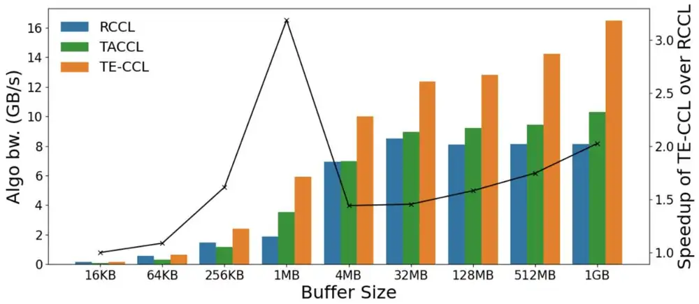
On DGX-1, DGX-2, NDv2 and two internal Microsoft topologies, the transfer times and bandwidths are the solver's own $\alpha$ – $\beta$ estimates, not hardware runs, so this page leaves them out. The measured numbers are an AMD testbed and solver run times. AMD testbed: two chassis of 16 GPUs, 32 in all, run AllGather on ROCm 6 against RCCL and TACCL (the paper's Figure 8). The GPU model, NIC and RCCL version are not named.

在 DGX-1、DGX-2、NDv2 與兩個 Microsoft 內部拓樸上，傳輸時間與頻寬都是求解器自己的 $\alpha$ – $\beta$ 估計，不是硬體實驗，所以本頁不列。實測的數字是一個 AMD 測試平台與求解器執行時間。AMD 測試平台：兩台各 16 顆 GPU 的機箱，共 32 顆，在 ROCm 6 上執行 AllGather，與 RCCL 及 TACCL 比較（論文 Figure 8）。論文沒有寫出 GPU 型號、NIC 與 RCCL 版本。

Comparison比較	Measured result實測結果
vs RCCL's ring, 1 MB output對 RCCL 的環，1 MB 輸出	about 3× faster約快 3 倍
vs RCCL, larger sizes對 RCCL，較大的大小	1.5–2× faster快 1.5–2 倍
vs TACCL對 TACCL	faster for most sizes多數大小都較快
Headline (abstract, §1)摘要與 §1 的主要數字	2.14× TACCL and 3.18× RCCL in algorithm bandwidth; the paper does not say whether these are means or maxima演算法頻寬為 TACCL 的 2.14 倍、RCCL 的 3.18 倍；論文沒有說明是平均還是最大值
Older ROCm 5.7較舊的 ROCm 5.7	larger gap at small sizes; the RCCL update narrowed it小大小時差距更大；RCCL 更新後縮小

Figure 8 of the TE-CCL paper: grouped bars of AllGather algorithm bandwidth for RCCL, TACCL and TE-CCL from 16 KB to 1 GB, with a line for TE-CCL's speed-up over RCCL on the right axis. — Figure 8 of the paper, measured on the 32-GPU AMD testbed (two chassis, ROCm 6). Bars: AllGather algorithm bandwidth of RCCL, TACCL and TE-CCL by buffer size (left axis). Line: TE-CCL's speed-up over RCCL (right axis), with its peak at 1 MB and 1.5–2× at larger buffers.論文的 Figure 8，在 32 GPU 的 AMD 測試平台（兩台機箱、ROCm 6）上實測。長條：RCCL、TACCL 與 TE-CCL 依緩衝區大小的 AllGather 演算法頻寬（左軸）。折線：TE-CCL 相對 RCCL 的加速（右軸），在 1 MB 達到高峰，較大緩衝區時為 1.5–2 倍。Screenshot of Liu et al., SIGCOMM 2024, Figure 8 (ACM PDF, p. 11).

The authors say they checked on these nodes that the solver's estimates match the hardware, but show no data. Solver run time at scale (Table 4); the epoch multiplier lengthens every epoch to save memory, and large AllToAlls still used about 350 GB of RAM:

作者說他們在這些節點上確認過求解器的估計與硬體相符，但沒有附上資料。大規模的求解器執行時間（Table 4）；epoch 倍數把每個 epoch 加長以節省記憶體，大型 AllToAll 仍用了約 350 GB RAM：

Topology拓樸	Collective, solver集體操作、求解器	GPUs (epoch multiplier)GPU 數（epoch 倍數）	Solve time求解時間
Internal 1內部 1	AllGather, A*	64 · 128	3,000 s · 7 h
Internal 2內部 2	AllGather, A*	128 · 256 (×2 at 256)128 · 256（256 時 ×2）	1,300 s · 2.8 h
Internal 1內部 1	AllToAll, LP	16 · 32 · 64 · 128 (×2 at 128)16 · 32 · 64 · 128（128 時 ×2）	66 · 215 · 500 · 800 s
Internal 2內部 2	AllToAll, LP	128 · 256 (×4 at 256)128 · 256（256 時 ×4）	2,600 · 1,500 s

The 256-GPU AllToAll solved faster than the 128-GPU one because its epochs were 4× longer. On small DGX-1 cases, TE-CCL solved every AllGather in at most 0.65 s, where SCCL needed more than a day; on an AllToAll with 8 chunks, SCCL timed out after 10,032.7 s and TE-CCL took 1.88 s. Against TACCL, solve times were on par: TE-CCL was faster in 27% to 83% of the scenarios. The A* solver cut a small AllGather from 346 s to 86.61 s; its loss in quality is again a model estimate.

256 GPU 的 AllToAll 比 128 GPU 的解得快，因為它的 epoch 長了 4 倍。在 DGX-1 的小案例上，TE-CCL 解每個 AllGather 最多 0.65 s，SCCL 則要一天以上；對 8 個 chunk 的 AllToAll，SCCL 在 10,032.7 s 後逾時，TE-CCL 只花 1.88 s。與 TACCL 相比求解時間相當：TE-CCL 在 27% 到 83% 的情境較快。A* 求解器把一個小型 AllGather 從 346 s 縮到 86.61 s；它損失多少品質，同樣只是模型估計。

6. Limits and open questions6. 限制與未解的問題

The paper's own limits (§8): failures inside a chassis are not handled; a cloud tenant may not know the topology, and profiled $\alpha$ and $\beta$ are unstable on a shared network; AllReduce runs only as ReduceScatter plus AllGather, without compute cost; lowering to a runtime is manual. A careful reader should add:

論文自己列出的限制（§8）：不處理機箱內部的故障；雲端租戶可能不知道拓樸，而在共享網路上量出的 $\alpha$ 與 $\beta$ 並不穩定；AllReduce 只能以 ReduceScatter 加 AllGather 執行，也不計計算成本；轉換到執行環境要靠手工。細心的讀者還應該補上：

Evidence. The only hardware result is one 32-GPU AMD system; the claim of about 2× better schedules than TACCL is a model estimate.證據。唯一的硬體結果是一套 32 GPU 的 AMD 系統；「排程比 TACCL 好約 2 倍」是模型估計。
Fixed inputs. A static topology and a demand known in advance; MoE all-to-all sizes are known only at run time.輸入固定。拓樸不變、需求事先已知；MoE all-to-all 的大小要到執行時才知道。
Cost of scale. Hours and about 350 GB of RAM at 128–256 GPUs; multi-tenant schedules are formulated but never run.規模的代價。128–256 顆 GPU 時需要數小時與約 350 GB RAM；多租戶排程只寫出模型，從未執行。

7. How it connects7. 與其他內容的關聯

Deep dive, sections 2 and 4 (with its Panel 4): epochs discretize the $\alpha$ – $\beta$ model, rounding latency up to whole epochs (try it in Panel 1), and the hierarchical and torus schedules are hand-made points in the space that the MILP searches.第 4 章第 2 與第 4 節（及其面板 4）：epoch 把 $\alpha$ – $\beta$ 模型離散化，把延遲取整到整數個 epoch（可在面板 1 試試），而階層式與環面排程都是 MILP 所搜尋空間中人工挑出的點。
SyCCL (next digest) applies this MILP only to small sub-demands; in its tests TE-CCL took 1,193 s on average for a 16-GPU AllGather and timed out at 512 GPUs. Theseus measured 13 hours before TE-CCL beat NCCL on a 32-GPU AllGather, so it accepts solver output while a job runs.SyCCL（下一篇導讀）只把這個 MILP 用在小的子需求上；在它的測試中，TE-CCL 解 16 GPU 的 AllGather 平均要 1,193 s，到 512 GPU 時逾時。Theseus 量到 TE-CCL 要 13 小時才在 32 GPU 的 AllGather 上勝過 NCCL，所以讓任務在執行中接收求解器的輸出。
Meta's RoCE paper used centralized traffic engineering to place flows, not to schedule chunks; it beat E-ECMP by 5–10% on 128 GPUs.Meta 的 RoCE 論文用集中式流量工程來放置流，而不是排程 chunk；在 128 顆 GPU 上比 E-ECMP 好 5–10%。

Key numbers關鍵數字

Number	數字	Meaning (measured)
2.14× / 3.18×	AllGather algorithm bandwidth over TACCL / RCCL, 32-GPU AMD testbed	32 GPU AMD 測試平台上，AllGather 演算法頻寬相對 TACCL / RCCL
≈ 3× ; 1.5–2×	Speed-up over RCCL at 1 MB ; at larger sizes (ROCm 6)	1 MB 時相對 RCCL 的加速 ; 較大大小時（ROCm 6）
≤ 0.65 s vs > 1 day	TE-CCL vs SCCL solve, DGX-1 AllGather with more than 3 chunks	TE-CCL 對 SCCL 的求解時間，DGX-1、超過 3 個 chunk 的 AllGather
1.88 s vs 10,032.7 s	TE-CCL solve vs SCCL timeout, AllToAll with 8 chunks	TE-CCL 求解對 SCCL 逾時，8 個 chunk 的 AllToAll
7 h ; 2.8 h	A* AllGather solve at 128 GPUs ; at 256 GPUs with 2× epochs	A* AllGather 在 128 GPU 的求解 ; 256 GPU、epoch 加長 2 倍
1,500 s	LP AllToAll solve at 256 GPUs with 4× epochs	LP AllToAll 在 256 GPU、epoch 加長 4 倍的求解
≈ 350 GB	Solver RAM for AllToAll on large topologies	大型拓樸上 AllToAll 的求解器記憶體

Terms used on this page本頁用到的術語

Time-expanded graph: One copy of every node per epoch, with link edges between epochs and buffer edges at GPUs.; 每個 epoch 都有每個節點的一份複本，epoch 之間有鏈路邊，GPU 上有緩衝邊。
Epoch: TE-CCL's time slot $\tau$ ; in most results, the fastest link's time for one chunk.; TE-CCL 的時間槽 $\tau$ ；多數結果中，是最快鏈路傳一個 chunk 的時間。
Commodity: One chunk of one source, flowing to the destinations that demand it.; 某個來源的一個 chunk，流向需要它的目的地。
Copy: A node keeps a chunk and forwards it on several links; modeled by a maximum over outgoing flows.; 節點留下 chunk 並從多條鏈路轉送；以外送流量的最大值建模。
MILP / LP: Linear program with or without integer variables; TE-CCL needs integers only when copy is used.; 有或沒有整數變數的線性規劃；TE-CCL 只有用到複製時才需要整數。
Algorithm bandwidth: Output buffer size divided by transfer time.; 輸出緩衝區大小除以傳輸時間。