Research digest 16 of 16 · Chapter 4: Collective communication

研究導讀 16 / 16 · 第 4 章：集體通訊

FAST: An Efficient Scheduler for All-to-All GPU CommunicationFAST：高效率的 GPU All-to-All 通訊排程器

NSDI 2026Yiran Lei, Dongjoo Lee, Liangyu Zhao, …, Justine Sherry, Eriko Nurvitadhi (Carnegie Mellon University, MangoBoost, University of Washington, University of Pennsylvania) · paper論文

After reading, you can explain how FAST schedules each skewed MoE all-to-all in microseconds: balance over NVLink, then one-to-one Birkhoff stages that keep the busiest server busy.讀完後，你能說明 FAST 如何在微秒內為每一次偏斜的 MoE all-to-all 排程：先用 NVLink 平衡，再用一對一的 Birkhoff 階段讓最忙的伺服器一直保持忙碌。

≈ 11 min · 1 interactive panel · 5-question quiz≈ 11 分鐘 · 1 個互動面板 · 5 題測驗Chapter 4 ↗第 4 章 ↗Jump to the quiz ↓跳到測驗 ↓

If you read nothing else

只讀這一段也可以

An MoE layer runs an all-to-all whose byte matrix is skewed and changes at every call. It crosses two tiers: NVLink inside a server, and NICs about ten times slower between servers. FAST computes a new schedule per call. Inside each server it balances bytes over NVLink, so that every GPU sends the same amount to the same-index GPU of each other server. Birkhoff's decomposition splits the remaining server-level matrix into one-to-one stages: no incast, and the busiest server never waits. Measured on 32 GPUs: MoE training 1.18–4.48× faster than RCCL (MI300X), skewed all-to-all 1.2–1.3× faster than NCCL (H200), and a 64-GPU schedule in 221 µs.

MoE 層執行的 all-to-all，位元組矩陣是偏斜的，而且每次呼叫都會變。它跨越兩層：伺服器內的 NVLink，以及伺服器之間慢了大約十倍的 NIC。FAST 每次呼叫都算出新的排程。在每台伺服器內，它先經 NVLink 平衡位元組，讓每顆 GPU 送給其他每台伺服器中相同索引的 GPU 一樣多的資料。Birkhoff 分解把剩下的伺服器層級矩陣拆成一對一的階段：沒有 incast，最忙的伺服器也從不等待。在 32 顆 GPU 上實測：MoE 訓練比 RCCL 快 1.18–4.48 倍（MI300X），偏斜的 all-to-all 比 NCCL 快 1.2–1.3 倍（H200），64 顆 GPU 的排程只需 221 µs。

Where this paper sits這篇論文的位置

Section 4.1 prices all-to-all at $\tfrac{N-1}{N}\,S$ per rank, which assumes equal blocks. Section 9.4 shows why expert parallelism (Section 3.7) breaks this: the router picks the top- $k$ experts of every token in every step, so the dispatch and combine all-to-alls are skewed, and their sizes are known only when the call starts.

第 4.1 節把 all-to-all 的成本定為每個 rank $\tfrac{N-1}{N}\,S$ ，前提是每個區塊一樣大。第 9.4 節說明專家平行（第 3.7 節）為什麼打破這一點：router 在每一步為每個 token 選出 top- $k$ 個專家，所以 dispatch 與 combine 兩次 all-to-all 都是偏斜的，而且大小要到呼叫開始時才知道。

Chapter 4 ends with an open question: how fast must a schedule be? Solvers write good schedules slowly; SyCCL needs about 37 minutes at 512 GPUs. Run-time libraries pick among fixed schedules: NCCL's PXN aggregates at the sender, DeepEP at the receiver, and Theseus switches to a NIC-balancing schedule above a skew threshold. FAST computes a schedule per call, in microseconds to milliseconds.

第 4 章最後留下一個問題：排程必須多快？求解器能寫出好排程，但很慢；SyCCL 在 512 顆 GPU 時需要約 37 分鐘。執行期的函式庫則在固定排程之間選擇：NCCL 的 PXN 在傳送端彙整，DeepEP 在接收端彙整，Theseus 在偏斜超過門檻時切換到平衡 NIC 的排程。FAST 每次呼叫都算一份排程，只需微秒到毫秒。

The problem, measured問題，用量測說明

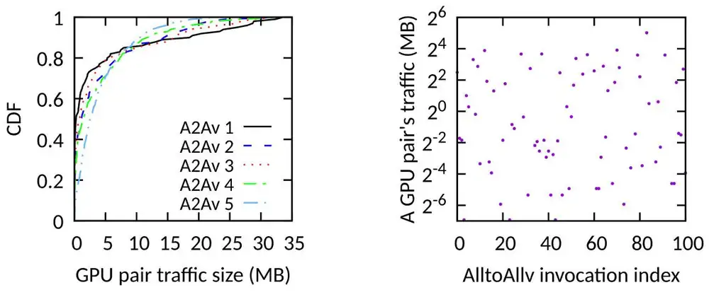
The authors profiled Megatron-LM pre-training of an MoE model with 32 experts, one per GPU (Figure 2 of the paper, below). The matrix is skewed: some GPU pairs exchange more than 12 times the median volume. It is also dynamic: the bytes of one pair change by orders of magnitude between calls, because the gate depends on the input. So the schedule must be computed online, per call.

作者剖析了 Megatron-LM 預訓練 MoE 模型的過程，32 個專家、每顆 GPU 一個（論文圖 2，見下）。矩陣是偏斜的：有些 GPU 對交換的量超過中位數的 12 倍。它也是動態的：同一對 GPU 的位元組數在呼叫之間相差好幾個數量級，因為 gate 取決於輸入。所以排程必須線上計算，每次呼叫算一次。

Figure 2 of the FAST paper. Left: CDF curves of GPU-pair traffic size from 0 to 35 MB for five all-to-all calls. Right: scatter of one GPU pair's traffic over 100 calls on a log scale. — Figure 2 of the paper (measured, Megatron-LM MoE pre-training, 32 experts on 32 GPUs). Left: CDF of bytes per GPU pair in five calls; a few pairs carry over 12 times the median. Right: one pair over 100 calls, on a log axis.論文圖 2（實測，Megatron-LM 預訓練 MoE，32 個專家、32 顆 GPU）。左：五次呼叫中每對 GPU 位元組數的 CDF；少數 GPU 對超過中位數的 12 倍。右：同一對 GPU 在 100 次呼叫中的流量，對數軸。USENIX NSDI '26, Lei et al., Figure 2 (captured from arXiv v3)

The fabric adds two problems. Per GPU, scale-up (inside a server) is about ten times faster than scale-out (between servers); the paper cites 900 GB/s for NVLink 5 against 800 Gb/s Ethernet. And transfers of 100 MB to 1 GB make incast, many senders to one receiver, a sustained congestion that DCQCN-style control does not remove.

網路再帶來兩個問題。以每顆 GPU 計，scale-up（伺服器內）比 scale-out（伺服器間）快大約十倍；論文引用 NVLink 5 的 900 GB/s 對比 800 Gb/s 的 Ethernet。而 100 MB 到 1 GB 的傳輸讓 incast（多個傳送端打向一個接收端）成為持續的壅塞，DCQCN 類的控制也消除不了。

Existing schedulers are too slow for this. In the paper's runs, TACCL needed more than 30 minutes for a balanced all-to-all on 32 GPUs, and SyCCL 3.6 s for 16 GPUs; both needed padded, balanced inputs. NCCL is fast, but its fixed schedule ignores skew.

現有的排程器太慢。在論文的實驗中，TACCL 為 32 顆 GPU 的平衡 all-to-all 需要超過 30 分鐘，SyCCL 為 16 顆 GPU 需要 3.6 秒；兩者都需要填補成平衡的輸入。NCCL 很快，但它固定的排程忽略了偏斜。

The design設計

1. One tier: one-to-one stages that keep the bottleneck busy1. 單層網路：讓瓶頸一直忙碌的一對一階段

Start with one tier: full bisection, bandwidth $B$ at every node, and $T_{ij}$ bytes from node $i$ to node $j$ . No schedule ends before the busiest sender or receiver has moved its bytes, so the bound is the largest row or column sum $L$ :

先看單層網路：完整二分頻寬、每個節點頻寬為 $B$ ， $T_{ij}$ 是節點 $i$ 送給節點 $j$ 的位元組。任何排程都要等最忙的傳送端或接收端送完才能結束，所以下界是最大的列或行總和 $L$ ：

\begin{gathered} t_{\text{opt}} = \frac{L}{B} \\ L = \max\Big(\max_i \sum_j T_{ij},\ \max_j \sum_i T_{ij}\Big) \end{gathered}

A schedule meets this bound if every stage is one-to-one (no incast) and the bottleneck node stays at line rate until it is done. Birkhoff's theorem (1946) gives such stages: a matrix with equal row and column sums is a weighted sum of permutation matrices. Each permutation is a stage, and its weight is the stage time. FAST first pads the lighter rows and columns with virtual entries, never sent, until every sum equals $L$ ; the bottleneck line gets none.

只要每個階段都是一對一（沒有 incast），而且瓶頸節點一直以線速傳到完成，排程就能達到這個下界。Birkhoff 定理（1946）給出這樣的階段：列與行總和都相等的矩陣，是置換矩陣的加權和。每個置換是一個階段，權重就是階段時間。FAST 先在較輕的列與行填上虛擬項（從不傳送），直到每個總和都等於 $L$ ；瓶頸那一列（或行）不會被填補。

MPI's classic SpreadOut uses fixed shifts: in stage $k$ , node $s$ sends to node $(s+k) \bmod N$ . It also avoids incast, but a stage lasts as long as its largest entry, so the bottleneck can wait. Figure 9 of the paper compares the two.

MPI 經典的 SpreadOut 使用固定位移：第 $k$ 個階段，節點 $s$ 送給節點 $(s+k) \bmod N$ 。它也沒有 incast，但一個階段要等最大的項傳完，所以瓶頸可能要等待。論文圖 9 比較這兩者。

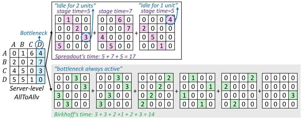
Figure 9 of the FAST paper: a 4 by 4 traffic matrix decomposed two ways, three SpreadOut stage matrices summing to 17 time units and six Birkhoff permutation matrices summing to 14. — Figure 9 of the paper (a design example, not a measurement). Server D must receive 14 units. SpreadOut's three shift stages take 17, because D idles in the first and last stage; Birkhoff's six one-to-one stages keep D busy and take 14.論文圖 9（設計範例，不是量測）。伺服器 D 必須接收 14 個單位。SpreadOut 的三個位移階段花 17，因為 D 在第一與最後一個階段閒置；Birkhoff 的六個一對一階段讓 D 一直忙碌，花 14。USENIX NSDI '26, Lei et al., Figure 9 (captured from arXiv v3)

The table checks the example, one question per row:

下表逐列驗算這個例子：

Question問題	Calculation算式	Result結果
Largest row sum: C sends最大列總和：C 送出	$4+5+0+3$	12A, B, D send 11 eachA、B、D 各送 11
Largest column sum: D receives最大行總和：D 接收	$4+7+3+0$	$14 = L$ A, B get 11, C gets 9; D is the bottleneckA、B 收 11，C 收 9；D 是瓶頸
SpreadOut: sum of each stage's largest entrySpreadOut：每個階段最大項的總和	$\max(1,2,3,5)+\max(6,7,4,5)+\max(4,2,5,1)$	$5+7+5 = 17$ units單位
Birkhoff: six stage weightsBirkhoff：六個階段的權重	$3+3+2+1+2+3$	$14 = L$
SpreadOut over BirkhoffSpreadOut 相對 Birkhoff	$17 \div 14$	$\approx 1.21$ 21% longer慢 21%

2. Two tiers: absorb the skew inside the server2. 兩層網路：在伺服器內吸收偏斜

On a real cluster each of the $m = 8$ GPUs of a server has its own NIC, so the busiest GPUs set the time. FAST uses the fast tier to fix this (§4.1, Figure 7). In one tile, server B sends to server A: B0 must send 8 units and B1 only 4, while A0 must receive 8 and A1 4. B0 first gives 2 units to B1 over scale-up. Each GPU then sends 6 units to the same-index GPU, which acts as a proxy. Finally A1 forwards 2 units to A0 over scale-up; this is the redistribution.

在實際的叢集上，一台伺服器的 $m = 8$ 顆 GPU 各有自己的 NIC，所以決定時間的是最忙的 GPU。FAST 用快的那一層解決這件事（§4.1、圖 7）。在一個區塊中，伺服器 B 送給伺服器 A：B0 要送 8 個單位、B1 只要 4 個，而 A0 要收 8 個、A1 收 4 個。B0 先經 scale-up 給 B1 2 個單位。接著每顆 GPU 送 6 個單位給相同索引的 GPU，由它充當代理。最後 A1 經 scale-up 轉 2 個單位給 A0；這就是重新分配（redistribution）。

The tile example of §4.1, in which bar width is NIC bytes. Without balancing, B0 sends 8 and A0 receives 8, while with FAST, after the NVLink moves of 2 units on each side, every NIC carries 6.依 §4.1 的區塊例子繪製，長條寬度是 NIC 上的位元組。未平衡時 B0 送 8、A0 收 8，而使用 FAST 時，經過兩側各 2 個單位的 NVLink 搬移，每張 NIC 都只承載 6。Drawn for this primer from §4.1 and Figure 7 of the paper

Now every tile is scalar-diagonal: GPU $k$ of one server sends the same bytes to GPU $k$ of another. A server's GPUs act as one, so the $mN \times mN$ GPU matrix becomes an $N \times N$ server matrix (Figure 8: 6×6 becomes 3×3). The price is extra scale-up bytes, which subsection 4 shows are cheap.

現在每個區塊都是純量對角的：一台伺服器的第 $k$ 顆 GPU 送給另一台第 $k$ 顆 GPU 的位元組都一樣多。同一台伺服器的 GPU 就像一個整體，所以 $mN \times mN$ 的 GPU 矩陣變成 $N \times N$ 的伺服器矩陣（圖 8：6×6 變成 3×3）。代價是多出的 scale-up 位元組，第 4 小節說明它們很便宜。

3. Server-level Birkhoff3. 伺服器層級的 Birkhoff

FAST then decomposes the server matrix by repeated perfect matchings on its nonzero entries: $O(N^3)$ per matching with the Hungarian algorithm, $O(N^5)$ in all. A balanced matrix needs $N$ stages, any matrix at most $N^2 - 2N + 2$ ; FAST does not seek the fewest, an NP-hard problem. Every GPU computes the same schedule from the same integer matrix, so no GPU sends schedules. Try both schedules in the panel.

FAST 接著在伺服器矩陣的非零項上反覆找完美匹配來分解它：用匈牙利演算法每次匹配 $O(N^3)$ ，總共 $O(N^5)$ 。平衡的矩陣需要 $N$ 個階段，任意矩陣最多 $N^2 - 2N + 2$ 個；FAST 不去找最少的階段數，那是 NP-hard 問題。每顆 GPU 都從同一個整數矩陣算出同一份排程，所以不必傳送排程。在面板中試試兩種排程。

Panel 1面板 1

Schedule a server-level all-to-all: SpreadOut or Birkhoff為伺服器層級的 all-to-all 排程：SpreadOut 或 Birkhoff

Matrix矩陣

Zipf skew

s

Zipf 偏斜

s

Servers

N

伺服器數

N

B_1 : B_2

per GPU每顆 GPU 的

B_1 : B_2

Random matrix隨機矩陣

Lower bound

L

下界

L

SpreadOut time

SpreadOut 時間

Birkhoff time

Birkhoff 時間

SpreadOut ÷ Birkhoff

FAST worst case ÷ optimum

FAST 最差情況 ÷ 最佳

Model: the matrix is in data units; time is units at one unit per tick. SpreadOut stage $k$ sends $s \to (s+k) \bmod N$ and lasts as long as its largest entry. Birkhoff pads the matrix to equal sums $L$ and peels off perfect matchings; its stages can differ from the paper's six, but the total is always $L$ . The coloured part of each stage is the time the bottleneck line moves real bytes. The last tile is Appendix A.1's bound $1 + (B_2/B_1)(m + m/n)$ with $m = 8$ and $n = N$ . Defaults: the paper's Figure 9 matrix (17 vs 14 units) and the H200 testbed's 9:1 ratio. The Zipf generator is ours (pair $r$ gets weight $1/r^s$ , mean 5 units), not the paper's. Try $s = 0$ : SpreadOut becomes optimal.

模型：矩陣以資料單位表示；時間以每單位一個時間刻度計。SpreadOut 第 $k$ 個階段傳送 $s \to (s+k) \bmod N$ ，持續到其中最大的項傳完。Birkhoff 把矩陣填補到總和都等於 $L$ ，再一層一層剝出完美匹配；它的階段可能與論文的六個不同，但總和永遠是 $L$ 。每個階段中上色的部分，是瓶頸那一列（或行）真正在傳位元組的時間。最後一格是附錄 A.1 的上界 $1 + (B_2/B_1)(m + m/n)$ ，其中 $m = 8$ 、 $n = N$ 。預設值：論文圖 9 的矩陣（17 對 14 個單位）以及 H200 實驗平台的 9:1 比例。Zipf 產生器是我們自己的（第 $r$ 對的權重為 $1/r^s$ ，平均 5 個單位），不是論文的。試試 $s = 0$ ：SpreadOut 就變成最佳。

4. The pipeline, and the worst case4. 管線，以及最差情況

Scale-up carries balancing, redistribution, and the intra-server part of the all-to-all. FAST balances first, then sorts the scale-out stages by size. Each stage's redistribution runs under the next stage, and the intra-server part runs beside stage 1, so only the last redistribution is exposed. Finer chunking gave little gain.

scale-up 承擔平衡、重新分配，以及 all-to-all 中伺服器內的部分。FAST 先平衡，再把 scale-out 階段依大小排序。每個階段的重新分配在下一個階段之下執行，伺服器內的部分與第 1 個階段並行，所以只有最後一次重新分配會露出來。切得更細收益很小。

The pipeline of §4.3, after Figure 11 of the paper. Stages S1–S3 grow in size, so each redistribution R

i

hides under the next stage, and only R3 is exposed.依 §4.3（論文圖 11）繪製的管線。階段 S1–S3 逐漸變大，所以每次重新分配 R

i

都藏在下一個階段之下，只有 R3 露出來。Drawn for this primer from §4.3 and Appendix A.1 of the paper

Appendix A.1 bounds the worst case for $n$ servers of $m$ GPUs, with scale-up bandwidth $B_1$ and scale-out bandwidth $B_2$ per GPU. The optimum for the server matrix is $t_{\text{opt}} = L/(mB_2)$ , and FAST is never worse than

附錄 A.1 給出最差情況的上界： $n$ 台伺服器、每台 $m$ 顆 GPU，每顆 GPU 的 scale-up 頻寬 $B_1$ 、scale-out 頻寬 $B_2$ 。伺服器矩陣的最佳時間是 $t_{\text{opt}} = L/(mB_2)$ ，而 FAST 不會比下式更差：

\frac{t_{\text{FAST}}}{t_{\text{opt}}} \le 1 + \frac{B_2}{B_1}\left(m + \frac{m}{n}\right)

The hiding needs $B_1 > (m-1)\,B_2$ , so that a stage's redistribution is shorter than the next stage. For the two testbeds:

隱藏需要 $B_1 > (m-1)\,B_2$ ，讓一個階段的重新分配比下一個階段短。兩個實驗平台的情況：

Question問題	Calculation算式	Result結果
H200: 450 GB/s NVLink, 400 Gb/s = 50 GB/s NIC, $m = 8$ , $n = 4$ H200：450 GB/s NVLink、400 Gb/s = 50 GB/s NIC、 $m = 8$ 、 $n = 4$	$1 + \tfrac{50}{450}\,(8 + 8/4)$	$\approx 2.11$ the paper reports 2.12×論文寫 2.12×
MI300X: 448 GB/s Infinity Fabric, 100 Gb/s = 12.5 GB/s NICMI300X：448 GB/s Infinity Fabric、100 Gb/s = 12.5 GB/s NIC	$1 + \tfrac{12.5}{448}\,(8 + 8/4)$	$\approx 1.28$
Hiding condition on H200H200 的隱藏條件	$450 > 7 \times 50 = 350$	holds成立

These are adversarial bounds. Measured, balancing and redistribution added under 5% of the scale-out time in most cases and under 8% at Zipf skew 0.9.

這些是對抗性的上界。實測中，平衡與重新分配在多數情況下增加不到 scale-out 時間的 5%，在 Zipf 偏斜 0.9 時不到 8%。

Implementation實作

FAST is one Python call, all_to_all_FAST, with the interface of PyTorch's all_to_all_single. On H200 it uses CUDA IPC for scale-up and NVSHMEM for scale-out; on MI300X it uses RCCL for both; CUDA streams run the pipeline. The scheduler runs on each GPU's host CPU. Its input is free: Megatron-LM already All-Gathers the per-expert token counts. The extra buffer is about 30% under random loads, under 0.22% of an H200's 141 GB. The code is public; the paper gives no line count.

FAST 是一個 Python 呼叫 all_to_all_FAST，介面與 PyTorch 的 all_to_all_single 相同。在 H200 上，scale-up 用 CUDA IPC、scale-out 用 NVSHMEM；在 MI300X 上兩者都用 RCCL；多個 CUDA stream 執行管線。排程器在每顆 GPU 的主機 CPU 上執行。它的輸入不需額外成本：Megatron-LM 本來就會 All-Gather 每個專家的 token 數。隨機負載下額外緩衝區約 30%，不到 H200 的 141 GB 的 0.22%。程式碼已公開；論文沒有給程式行數。

What was measured量了什麼

Two testbeds of 4 servers × 8 GPUs, one NIC per GPU, 100 MB to 1 GB per GPU. Loads are random or Zipf-skewed; profiled MoE traces show skew factors of 0.4–0.8. The metric is algorithmic bandwidth, total bytes over GPUs times completion time; with 25% intra-server bytes the H200 optimum is $50/0.75 \approx 66.7$ GB/s.

兩個實驗平台，各 4 台 × 8 顆 GPU，每顆 GPU 一張 NIC，每顆 GPU 傳 100 MB 到 1 GB。負載為隨機或 Zipf 偏斜；剖析過的 MoE 軌跡偏斜係數為 0.4–0.8。指標是演算法頻寬：總位元組除以 GPU 數乘完成時間；若 25% 的位元組在伺服器內，H200 的最佳值是 $50/0.75 \approx 66.7$ GB/s。

Testbed平台	Scale-up per GPU每顆 GPU 的 scale-up	Scale-out per GPU每顆 GPU 的 scale-out	Baselines比較對象
32 H200 (4 × 8)32 顆 H200（4 × 8）	NVLink, 450 GB/s (9:1)NVLink，450 GB/s（9:1）	400 Gb/s InfiniBand, credit-based flow control, 4 KB MTU400 Gb/s InfiniBand，credit-based 流量控制，4 KB MTU	NCCL 2.27.3, DeepEP, MSCCL, TACCL, TE-CCL
32 MI300X (4 × 8)32 顆 MI300X（4 × 8）	Infinity Fabric full mesh, 448 GB/s (35:1)Infinity Fabric 全連接網格，448 GB/s（35:1）	100 Gb/s RoCEv2, DCQCN as shipped, 1 KB MTU100 Gb/s RoCEv2，出廠設定的 DCQCN，1 KB MTU	RCCL, SpreadOut, MSCCL, TACCL, TE-CCL

FAST's speedup over each baseline:

FAST 相對各比較對象的加速：

Testbed and workload平台與負載	FAST's speedupFAST 的加速
H200, randomH200，隨機	NCCL 1.01–1.1×, DeepEP 1.5–1.9×, TACCL 1.5–1.7×NCCL 1.01–1.1×、DeepEP 1.5–1.9×、TACCL 1.5–1.7×
H200, Zipf 0.8H200，Zipf 0.8	NCCL 1.2–1.3×, DeepEP 1.2–1.5×, TACCL more than 3×NCCL 1.2–1.3×、DeepEP 1.2–1.5×、TACCL 超過 3×
MI300X, randomMI300X，隨機	RCCL 1.1–10×, SpreadOut 1.9–2.1×, TACCL 1.3–1.8×, TE-CCL 1.6–2.3×RCCL 1.1–10×、SpreadOut 1.9–2.1×、TACCL 1.3–1.8×、TE-CCL 1.6–2.3×
MI300X, Zipf 0.8MI300X，Zipf 0.8	RCCL 1.3–2.6×, SpreadOut 2.5–2.8×, TACCL 2.9–3.8×, TE-CCL 3.6–4.7×RCCL 1.3–2.6×、SpreadOut 2.5–2.8×、TACCL 2.9–3.8×、TE-CCL 3.6–4.7×
MI300X, Zipf 0.3–0.9MI300X，Zipf 0.3–0.9	RCCL 1.6–10×, SpreadOut 2.1–3.1×, TACCL 2.1–4.5×; within 1.08× of optimalRCCL 1.6–10×、SpreadOut 2.1–3.1×、TACCL 2.1–4.5×；距最佳在 1.08 倍以內

NCCL's PXN aggregates at the sender, which smooths mild skew; DeepEP aggregates at the receiver, so skew makes GPUs contend for one GPU's NVLink. Solvers waste stages on padding, and RCCL, with no schedule, loses to incast as transfers grow. On a balanced all-to-all FAST gains nothing: DeepEP 60 GB/s, TACCL 59, NCCL and FAST 58.

NCCL 的 PXN 在傳送端彙整，能撫平輕微偏斜；DeepEP 在接收端彙整，所以偏斜讓好幾顆 GPU 搶同一顆 GPU 的 NVLink。求解器把階段浪費在填補上，而沒有排程的 RCCL 隨傳輸變大輸給 incast。在平衡的 all-to-all 上 FAST 沒有增益：DeepEP 60 GB/s、TACCL 59、NCCL 與 FAST 58。

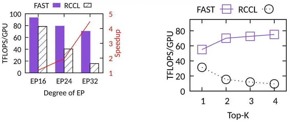
Training. Megatron-LM MoE training ran on the MI300X testbed with FAST for every all-to-all, against PyTorch's all_to_all_single over RCCL (solvers cannot run per call). With top-2 routing, FAST was 1.18× faster at EP16 and 4.48× at EP32. RCCL falls fast because a receiving GPU takes up to 8 concurrent remote flows at EP16 and up to 24 at EP32. At EP32 with top- $k$ from 1 to 4 the speedup was 1.75–7.88×: larger flows amortize FAST's staging, while RCCL meets more collisions.

訓練。在 MI300X 平台上以 Megatron-LM 訓練 MoE，每次 all-to-all 都用 FAST，比較基準是 PyTorch 的 all_to_all_single 搭配 RCCL（求解器無法每次呼叫都執行）。在 top-2 路由下，FAST 在 EP16 快 1.18 倍，在 EP32 快 4.48 倍。RCCL 下降得快，因為一顆接收 GPU 在 EP16 最多同時承接 8 條遠端流，在 EP32 最多 24 條。在 EP32、top- $k$ 從 1 到 4 時，加速是 1.75–7.88 倍：較大的流攤平了 FAST 的暫存成本，而 RCCL 遇到更多碰撞。

Figure 15 of the FAST paper. Left: bar chart of TFLOPS per GPU for FAST and RCCL at EP16, EP24 and EP32 with a speedup line. Right: TFLOPS per GPU against top-k from 1 to 4 for FAST and RCCL. — Figure 15 of the paper (measured, Megatron-LM MoE training on 32 MI300X, 100 Gb/s RoCEv2 per GPU). Left: EP16–EP32 with top-2; the red line is the speedup over RCCL, 1.18× to 4.48×. Right: EP32 with top- $k$ from 1 to 4.論文圖 15（實測，在 32 顆 MI300X 上以 Megatron-LM 訓練 MoE，每顆 GPU 100 Gb/s RoCEv2）。左：top-2 下的 EP16–EP32；紅線是相對 RCCL 的加速，1.18× 到 4.48×。右：EP32、top- $k$ 從 1 到 4。USENIX NSDI '26, Lei et al., Figure 15 (captured from arXiv v3)

Scheduling time, measured on the host CPU: 3.1 µs for 16 GPUs (SyCCL: 3.6 s), 25 µs for 32, 221 µs for 64, 805 µs for 96, and 77 ms for 320. Earlier solvers generally fail beyond 64 GPUs.

排程時間，在主機 CPU 上量測：16 顆 GPU 3.1 µs（SyCCL：3.6 秒），32 顆 25 µs，64 顆 221 µs，96 顆 805 µs，320 顆 77 ms。較早的求解器一般在超過 64 顆 GPU 時就失敗。

Measured schedule times, log axis. Green: FAST (§4.4, Figure 16). Red: SyCCL and TACCL in this paper; pale: SyCCL at 512 GPUs, from its own paper. The orange line marks one EP64 all-to-all of 1 GB per GPU at 400 Gb/s, and the band shows how often MoE traffic shifts (abstract).實測的排程時間，對數軸。綠色：FAST（§4.4、圖 16）。紅色：本論文中的 SyCCL 與 TACCL；淡色：SyCCL 論文自己在 512 顆 GPU 的時間。橘色線標出每顆 GPU 1 GB、400 Gb/s 的一次 EP64 all-to-all，色帶則是 MoE 流量變化的頻率（摘要）。Drawn for this primer from §4.4, §5.1 and §5.3 of the paper and the collectives research notes, 9.1

The paper's budget example:

論文的預算例子：

Question問題	Calculation算式	Result結果
Shortest EP64 all-to-all, 1 GB per GPU at 400 Gb/s = 50 GB/sEP64 all-to-all 的最短時間，每顆 GPU 1 GB、400 Gb/s = 50 GB/s	$1\ \text{GB} \div 50\ \text{GB/s}$	$\ge 20$ ms
FAST's 64-GPU schedule as a share of itFAST 的 64 顆 GPU 排程佔其比例	$0.221\ \text{ms} \div 20\ \text{ms}$	$\approx 1.1\%$
SyCCL's 16-GPU solve against FAST'sSyCCL 的 16 顆 GPU 求解相對 FAST	$3.6\ \text{s} \div 3.1\ \mu\text{s}$	$\approx 1.2 \times 10^{6}$ six orders of magnitude六個數量級

Section 5.4 studies 300 GPUs and other bandwidth ratios in a simulator, so this page leaves its numbers out.

第 5.4 節用模擬器研究 300 顆 GPU 與其他頻寬比例，所以本頁不列出它的數字。

Limits and open questions限制與未解的問題

Scale. All measured transfers and training use 32 GPUs; at 320 GPUs a 77 ms schedule is no longer small next to a 20 ms transfer. Topology. FAST assumes two tiers with a full-bisection scale-out tier; multi-tier networks and asymmetric scale-up (MI250 ring, V100 cube mesh) are untested, and the switches are not described. Sharing. The all-to-all is assumed to have the network to itself. Evidence. The large training gain is against RCCL on 100 Gb/s RoCE with stock DCQCN; on H200 the skewed gain over NCCL is 1.2–1.3×, with no training run. The trained model's size is not given. The authors call FAST orthogonal to congestion control: it removes incast by design.

規模。所有實測的傳輸與訓練都只用 32 顆 GPU；在 320 顆 GPU 時，77 ms 的排程相對 20 ms 的傳輸已不算小。拓樸。FAST 假設兩層網路，且 scale-out 層具完整二分頻寬；多層網路與非對稱的 scale-up（MI250 的環、V100 的 cube mesh）都未測試，論文也沒有描述交換器。共用。它假設 all-to-all 獨佔網路。證據。大幅的訓練增益是對比在 100 Gb/s RoCE、出廠 DCQCN 上的 RCCL；在 H200 上，偏斜負載相對 NCCL 的增益是 1.2–1.3 倍，而且沒有訓練實驗。論文也沒有給訓練模型的大小。作者認為 FAST 與壅塞控制正交：它在設計上就消除 incast。

How it connects與其他內容的關聯

Section 9.4 of the chapter lists answers to MoE skew; FAST is the one that computes a schedule per call. Theseus switches from a menu of compiled schedules to a NIC-balancing one when the predicted skew passes 1.4. NCCLX's AllToAllvDynamic reads split sizes in GPU memory; FAST needs them on the host, from Megatron-LM's All-Gather. PReCCL relays one slow pair through a GPU of the same node, a small form of balancing. The same-index proxy is the rail idea of Rail-only and PXN. TE-CCL and SyCCL solve fixed demands near-optimally; FAST trades generality for speed. MixNet attacks the same skew with reconfigurable optics, and UBEP the all-to-all of large scale-up domains.

第 4 章第 9.4 節列出應對 MoE 偏斜的方法；FAST 是每次呼叫都算排程的那一種。Theseus 在預測偏斜超過 1.4 時，從編譯好的排程選單切換到平衡 NIC 的排程。NCCLX 的 AllToAllvDynamic 從 GPU 記憶體讀取切分大小；FAST 則需要在主機上知道大小，由 Megatron-LM 的 All-Gather 提供。PReCCL 讓一對變慢的 GPU 經同節點的另一顆 GPU 轉送，是平衡的小型版本。相同索引的代理就是 Rail-only 與 PXN 的 rail 概念。TE-CCL 與 SyCCL 為固定需求求出接近最佳的解；FAST 以通用性換取速度。MixNet 用可重組的光學元件處理同樣的偏斜，UBEP 則處理大型 scale-up 網域中的 all-to-all。

Key numbers關鍵數字

Number數字	What was measured (4 servers × 8 GPUs unless noted)量了什麼（除非註明，皆為 4 台 × 8 顆 GPU）
1.2–1.3×	Skewed all-to-all (Zipf 0.8) vs NCCL, H200, 400 Gb/s InfiniBand偏斜 all-to-all（Zipf 0.8）相對 NCCL，H200、400 Gb/s InfiniBand
2.5–4.7×	Skewed all-to-all vs SpreadOut, TACCL and TE-CCL, MI300X, 100 Gb/s RoCEv2偏斜 all-to-all 相對 SpreadOut、TACCL 與 TE-CCL，MI300X、100 Gb/s RoCEv2
1.18–4.48×	Megatron-LM MoE training vs RCCL, EP16–EP32, top-2, MI300XMegatron-LM MoE 訓練相對 RCCL，EP16–EP32、top-2、MI300X
1.75–7.88×	Same, EP32, top- $k$ from 1 to 4同上，EP32、top- $k$ 從 1 到 4
< 5% (< 8%)	Balancing and redistribution over scale-out time, most cases (Zipf 0.9), MI300X平衡與重新分配佔 scale-out 時間，多數情況（Zipf 0.9），MI300X
3.1 µs / 3.6 s	Schedule time for 16 GPUs, FAST / SyCCL16 顆 GPU 的排程時間，FAST／SyCCL
221 µs / 77 ms	FAST schedule time for 64 / 320 GPUs (host CPU)FAST 為 64／320 顆 GPU 排程的時間（主機 CPU）

Terms used on this page本頁用到的術語

Scale-up / scale-out: The fast tier inside a server (NVLink, Infinity Fabric) / the slower tier between servers (NICs and switches).; 伺服器內的快速層（NVLink、Infinity Fabric）／伺服器之間較慢的層（NIC 與交換器）。
SpreadOut: MPI's shift schedule: in stage $k$ , node $s$ sends to node $(s+k) \bmod N$ .; MPI 的位移排程：第 $k$ 個階段，節點 $s$ 送給節點 $(s+k) \bmod N$ 。
Birkhoff decomposition: Writing a matrix with equal row and column sums as a weighted sum of permutation matrices.; 把列總和與行總和都相等的矩陣寫成置換矩陣的加權和。
Redistribution: The scale-up step after a stage that moves bytes from the proxy GPU to their real destination.; 每個階段之後的 scale-up 步驟，把位元組從代理 GPU 搬到真正的目的地。
Algorithmic bandwidth: Total bytes divided by the number of GPUs times the completion time.; 總位元組除以 GPU 數乘完成時間。