Research digest 2 of 16 · Chapter 4: Collective communication

研究導讀 2 / 16 · 第 4 章：集體通訊

SyCCL: Exploiting Symmetry for Efficient Collective Communication SchedulingSyCCL：利用對稱性實現高效的集體通訊排程

SIGCOMM 2025Jiamin Cao, Shangfeng Shi, Jiaqi Gao et al. (Alibaba Cloud, Tsinghua University) · paper論文

After reading, you can explain how SyCCL uses symmetry in collectives and fabrics to cut schedule synthesis from hours to seconds, and why its testbed gains shrink to a few percent per step.讀完後，你能說明 SyCCL 如何利用集體操作與網路的對稱性，把排程合成從數小時縮短到數秒，以及為什麼它在測試平台上的增益到了每個訓練步驟只剩幾個百分點。

≈ 11 min · 1 interactive panel · 5-question quiz≈ 11 分鐘 · 1 個互動面板 · 5 題測驗Chapter 4 ↗第 4 章 ↗Jump to the quiz ↓跳到測驗 ↓

If you read nothing else

只讀這一段也可以

NCCL's ring and tree ignore the fabric; TE-CCL's solver fits it but takes hours and timed out at 512 GPUs. SyCCL uses symmetry: an AllGather is N relabeled copies of one broadcast, and a cluster's servers or rails form identically wired groups. It plans a collective as a sketch of small sub-demands inside groups, solves one per isomorphism class with TE-CCL's MILP, mixes sketches so each tier's load matches its bandwidth, and simulates candidates to keep the fastest. Synthesis took at most 29.8 s up to 64 GPUs and about 37 minutes at 512. On a 32-GPU testbed, bus bandwidth rose by up to 108% over NCCL, but iterations got only 0.4–6.3% faster.

NCCL 的環與樹不理會網路結構；TE-CCL 的求解器貼合網路，但要花數小時，到 512 顆 GPU 時逾時。SyCCL 利用對稱性：AllGather 是同一次廣播重新編號後的 N 份複本，叢集裡的伺服器或 rail 構成接線相同的群組。它把集體操作規劃成由群組內小子需求組成的 sketch，用 TE-CCL 的 MILP 為每個同構類別只解一個，混合多個 sketch 讓每一層的負載配合它的頻寬，再模擬各候選、留下最快的。合成在 64 顆 GPU 以內最多 29.8 s，512 顆時約 37 分鐘。在 32 GPU 測試平台上，匯流排頻寬比 NCCL 最多高 108%，迭代卻只快 0.4–6.3%。

1. Where this paper sits1. 這篇論文的位置

Section 4.4 shows that a server is two networks, NVLink inside and NICs outside, and that a hand-made hierarchical schedule splits the work between them. Section 9.1 introduces schedule synthesis, and the previous digest, TE-CCL, gives its exact model: one MILP over the whole cluster, which needs hours at 128–256 GPUs. What was missing is a way to keep a solver's fit to the fabric at cluster scale. SyCCL (Alibaba Cloud and Tsinghua University) finds it in symmetry.

第 4.4 節說明一台伺服器是兩個網路：內部是 NVLink，外部是 NIC，而人工設計的階層式排程把工作分給兩者。第 9.1 節介紹排程合成，上一篇導讀 TE-CCL 給出它的精確模型：對整個叢集建一個 MILP，在 128–256 顆 GPU 時要花數小時。缺少的是一種在叢集規模下仍保有求解器貼合網路能力的方法。SyCCL（Alibaba Cloud 與清華大學）在對稱性中找到它。

2. The problem, measured2. 問題，用量測說話

The paper's sharpest motivation is an analysis with its production parameters (§2.1). In Alibaba's H800 cluster each GPU has 180 GB/s of NVLink and one 400 Gb/s (50 GB/s) NIC, a ratio of 3.6 to 1. NCCL's ring AllGather chains a server's 8 GPUs and joins the chains, so it crosses 7 NVLink hops for each network hop (Figure 1). It implicitly assumes a 7 to 1 ratio. NVLink then sets the pace, and the NIC waits:

論文最有力的動機，是一段使用其生產參數的分析（§2.1）。在 Alibaba 的 H800 叢集中，每顆 GPU 有 180 GB/s 的 NVLink 與一張 400 Gb/s（50 GB/s）的 NIC，比例是 3.6 比 1。NCCL 的環形 AllGather 把一台伺服器的 8 顆 GPU 串成鏈，再把各鏈接起來，所以每跳一次網路就要跳 7 次 NVLink（圖 1）。它隱含假設比例是 7 比 1。於是 NVLink 決定步調，NIC 只能等待：

Question問題	Calculation算式	Result結果
NVLink-to-NIC bandwidth per GPU每顆 GPU 的 NVLink 對 NIC 頻寬	$180 \div 50$	$3.6 : 1$
Share of time the NIC idlesNIC 閒置的時間比例	$(7 - 3.6) \div 7$	$\approx 48.6\%$ the paper writes 48.5%論文寫作 48.5%
Waste of all bandwidth: the NIC is 1 of 4.6 units占全部頻寬的浪費：NIC 是 4.6 單位中的 1	$48.6\% \div (3.6 + 1)$	$\approx 10.6\%$

Figure 1. The paper's Figure 2 argument, redrawn: per unit of data, 7 NVLink hops at 180 GB/s take longer than 1 NIC hop at 50 GB/s, so the NIC is busy

3.6/7

of the time. The numbers follow from the production parameters of an H800 server.圖 1。重畫論文 Figure 2 的論證：每單位資料，以 180 GB/s 走 7 跳 NVLink，比以 50 GB/s 走 1 跳 NIC 更久，所以 NIC 只有

3.6/7

的時間在忙。這些數字由 H800 伺服器的生產參數推算而來。Drawn for this primer from Cao et al., SIGCOMM 2025, §2.1 and Figure 2.

At small sizes the problem is the hop count: per the paper, NCCL can be 4× worse there than synthesized schedules. Synthesizers fix both problems but do not scale: as the paper reports, SCCL needed more than 24 hours for a 16-GPU AllGather, and in SyCCL's own runs TE-CCL averaged 1,193 s for one (Table 5).

小訊息時，問題在跳數：依論文所述，NCCL 在這裡可能比合成的排程差 4 倍。合成器能解決這兩個問題，卻無法擴大規模：依論文的引述，SCCL 對 16 GPU 的 AllGather 需要超過 24 小時，而在 SyCCL 自己的實驗中，TE-CCL 解一個平均要 1,193 s（Table 5）。

3. The design3. 設計

3.1 Two kinds of symmetry3.1 兩種對稱

Collective symmetry. In a one-to-all collective every non-source GPU wants the same data. An AllGather is N broadcasts, an AllToAll N scatters, a ReduceScatter N reduces, and they are isomorphic: relabel the GPUs and one becomes another. Topology symmetry. SyCCL splits the fabric into dimensions, one per kind of connection (NVSwitch, leaf, spine), found automatically. Each GPU belongs to one group per dimension, and the groups of a dimension are isomorphic (Figure 2).

集體操作的對稱。在一對多的集體操作中，每顆非來源 GPU 想要的資料都一樣。AllGather 是 N 次廣播，AllToAll 是 N 次 scatter，ReduceScatter 是 N 次 reduce，而且它們彼此同構（isomorphic）：把 GPU 重新編號，一個就變成另一個。拓樸的對稱。SyCCL 把網路切成維度（dimension），每種連線一個維度（NVSwitch、leaf、spine），並自動找出它們。每顆 GPU 在每個維度屬於一個群組（group），同一維度的群組彼此同構（圖 2）。

Figure 2. Two-level decomposition (§3.1, the paper's Figure 3). Left: four of the 16 broadcasts in an AllGather, each the same problem with the GPUs renumbered. Right: GPU

4s + j

sits in server

s

on rail

j

; the blue rows are dimension-0 groups, while the orange-outlined columns are dimension-1 groups.圖 2。兩層分解（§3.1，論文 Figure 3）。左：AllGather 中 16 次廣播的其中四次，每次都是同一個問題，只是 GPU 重新編號。右：GPU

4s + j

位於伺服器

s

、rail

j

；藍色橫列是維度 0 的群組，橘色框起的直行則是維度 1 的群組。Drawn for this primer from Cao et al., SIGCOMM 2025, §3.1 and Figure 3.

3.2 Sketches, and solving one sub-demand per class3.2 Sketch，以及每類只解一個子需求

A sketch has $K$ stages. Stage $k$ holds sub-demands $R_{k,d,g}$ : sources send to receivers inside group $g$ of dimension $d$ . Sources must already hold the data, and every GPU becomes a destination exactly once. In the paper's Figure 5, a broadcast from GPU 0 sends $\{0\}\to\{1,2,3\}$ inside the server and $\{0\}\to\{4,8,12\}$ along the rail at once; stage 1 broadcasts inside the other three servers. A MILP fills in each sub-schedule, and the best combination becomes a schedule candidate (the paper's Figure 5, below).

sketch 有 $K$ 個階段。階段 $k$ 包含子需求（sub-demand） $R_{k,d,g}$ ：來源在維度 $d$ 的群組 $g$ 內送給接收者。來源必須已經持有資料，每顆 GPU 恰好成為一次目的地。在論文的 Figure 5 中，從 GPU 0 出發的廣播同時在伺服器內送 $\{0\}\to\{1,2,3\}$ 、沿 rail 送 $\{0\}\to\{4,8,12\}$ ；階段 1 再在另外三台伺服器內廣播。由 MILP 填入每個子排程，最佳的組合成為一個排程候選（見下方論文的 Figure 5）。

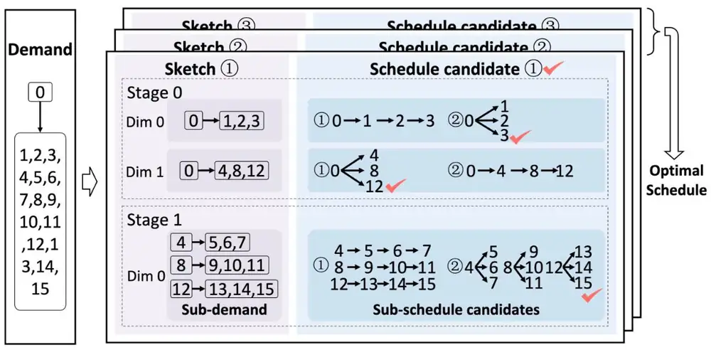
Figure 5 of the SyCCL paper: a broadcast from GPU 0 to GPUs 1 to 15 split by sketches into stages and dimensions, each sub-demand with chain or tree sub-schedule candidates, the chosen ones ticked. — Figure 5 of the paper (an algorithm diagram). Sketch ① splits the broadcast from GPU 0 into stages and dimensions; each sub-demand has chain or tree sub-schedules, the ticked ones form candidate ①, and the best sketch wins.論文的 Figure 5（演算法示意圖）。sketch ① 把從 GPU 0 出發的廣播依階段與維度拆開；每個子需求有鏈或樹的子排程，打勾的組成候選 ①，最佳的 sketch 勝出。Screenshot of Cao et al., SIGCOMM 2025, Figure 5 (author PDF, p. 4).

Four of the five sub-demands are one-to-three broadcasts inside a server, so SyCCL solves one and maps it onto the others (Figure 3).

五個子需求中有四個是伺服器內的一對三廣播，所以 SyCCL 只解一個，再對應到其他的（圖 3）。

Figure 3. Symmetry collapses the search: the paper's Figure 5 sketch has five sub-demands in two isomorphism classes, so two small MILPs replace one over all 16 GPUs.圖 3。對稱性讓搜尋塌縮：論文 Figure 5 的 sketch 有五個子需求、分屬兩個同構類別，所以兩個小 MILP 取代了涵蓋全部 16 顆 GPU 的一個 MILP。Drawn for this primer from Cao et al., SIGCOMM 2025, Figure 5, Table 4 and §5.3.

The search enumerates, per stage, the dimensions, groups, and source and receiver sets. Three rules prune it: isomorphic sketches count once; isomorphic groups in a stage must have the same receiver-to-source ratio, because the paper expects optimal schedules to treat them alike; and a Scatter visits each dimension at most once. The second rule is an expectation, not a proof.

搜尋在每個階段列舉維度、群組，以及來源與接收者集合。三條規則負責剪枝：同構的 sketch 只算一次；同一階段中同構群組的接收者對來源比例必須相同，因為論文預期最佳排程會一視同仁地對待它們；Scatter 對每個維度最多經過一次。第二條規則是一種預期，不是證明。

3.3 Matching each tier's load to its bandwidth3.3 讓每一層的負載配合它的頻寬

One sketch rarely loads the tiers in proportion to their bandwidth: the Figure 5 sketch puts 12 receptions on dimension 0 and 3 on dimension 1. SyCCL first replicates a sketch with GPU and group mappings so that isomorphic groups carry equal load. It then mixes such combinations with chunk fractions $t_i$ , chosen so that each dimension's share of the workload $w$ equals its share $u_d$ of the bandwidth:

單一 sketch 很少能依頻寬比例分配各層的負載：Figure 5 的 sketch 在維度 0 上有 12 次接收，在維度 1 上只有 3 次。SyCCL 先以 GPU 與群組的對應複製 sketch，讓同構群組承擔相同的負載。接著以 chunk 比例 $t_i$ 混合這些組合，讓每個維度在工作量 $w$ 中的占比等於它在頻寬中的占比 $u_d$ ：

\frac{\sum_i t_i\, w_{i,d}}{\sum_i \sum_{d'} t_i\, w_{i,d'}} = u_d \quad \forall d, \qquad \sum_i t_i = 1

Candidates without a valid solution are dropped. The paper's example mixes combination $C_4$ (4 sketches, workload 21:6) with $C_5$ (7 sketches, 3:24) on links with capacities 4:5:

沒有有效解的候選會被丟棄。論文的例子把組合 $C_4$ （4 個 sketch、工作量 21:6）與 $C_5$ （7 個 sketch、3:24）混合，鏈路容量比為 4:5：

Question問題	Calculation算式	Result結果
Workload of the mix with half the data each各分一半資料時的總工作量	$\tfrac12(21 + 3) : \tfrac12(6 + 24)$	$12 : 15 = 4 : 5$ matches the capacities與容量相符
Data per sketch in $C_4$ $C_4$ 中每個 sketch 的資料	$\tfrac12 \div 4$	$1/8$
Data per sketch in $C_5$ $C_5$ 中每個 sketch 的資料	$\tfrac12 \div 7$	$1/14$

This is the fix for the ring's waste: change how the data is split across tiers, not the links. AllToAll and reductions reuse the method, and AllReduce is a ReduceScatter followed by an AllGather.

這就是解決環形浪費的方法：改變資料在各層之間的切分，而不是改變鏈路。AllToAll 與歸約類操作沿用同一方法，AllReduce 則是 ReduceScatter 之後接 AllGather。

3.4 Solve small, merge, simulate3.4 小規模求解、合併、模擬

Sub-demands of the same group and stage compete for links, so SyCCL solves them together as one MILP borrowed from TE-CCL: epochs $\tau$ , a chunk of size $s$ needs $\alpha + \beta s$ per link, so the next hop starts $\lceil (\alpha + \beta s)/\tau \rceil$ epochs later, and the objective is the fewest epochs. Isomorphic groups reuse one solution, and independent MILPs run in parallel. Stage times cannot simply be added: in the paper's Figure 12, sub-schedules of $5\tau$ , $4\tau$ and $5\tau$ sum to $10\tau$ , but stage-1 sends start as soon as their chunks arrive, and an event simulator built on ASTRA-sim, with the same $\alpha$ – $\beta$ model, gives $9\tau$ . SyCCL simulates every merged candidate and keeps the fastest.

同一群組、同一階段的子需求會競爭鏈路，所以 SyCCL 把它們合成一個借自 TE-CCL 的 MILP 一起求解：以 epoch $\tau$ 計時，大小 $s$ 的 chunk 每條鏈路需要 $\alpha + \beta s$ ，所以下一跳在 $\lceil (\alpha + \beta s)/\tau \rceil$ 個 epoch 後才開始，目標是 epoch 數最少。同構群組重用同一個解，獨立的 MILP 平行求解。各階段時間不能直接相加：在論文的 Figure 12 中， $5\tau$ 、 $4\tau$ 與 $5\tau$ 的子排程加起來是 $10\tau$ ，但階段 1 的傳送在 chunk 一到就開始，建在 ASTRA-sim 上、使用相同 $\alpha$ – $\beta$ 模型的事件模擬器算出 $9\tau$ 。SyCCL 模擬每個合併後的候選，留下最快的。

Synthesis runs in two steps. A coarse pass with long epochs ( $E_1 = 3.0$ ) scores every candidate; candidates more than $R_1 = 20\%$ worse than the best are dropped, and at most $R_2 = 8$ get a fine pass ( $E_2 = 0.5$ , or 1.0 at 512 GPUs). Panel 1 counts what symmetry removes from the problem.

合成分兩步。粗略的一輪用長 epoch（ $E_1 = 3.0$ ）為每個候選打分；比最佳者差超過 $R_1 = 20\%$ 的被丟棄，最多 $R_2 = 8$ 個進入精細的一輪（ $E_2 = 0.5$ ，512 GPU 時為 1.0）。面板 1 計算對稱性從問題中拿掉了多少。

Panel 1面板 1

What symmetry removes from the search對稱性從搜尋中拿掉了什麼

Servers

S

伺服器數

S

GPUs per server

g

每台伺服器的 GPU 數

g

Chunks per GPU

C

每顆 GPU 的 chunk 數

C

GPUs

N = S g

GPU 數

N = S g

Sub-demands in the AllGather

AllGather 的子需求數

MILPs actually solved

實際求解的 MILP 數

TE-CCL: one MILP, variables

TE-CCL：一個 MILP 的變數

SyCCL: largest MILP, variables

SyCCL：最大 MILP 的變數

Measured mean synthesis

實測平均合成時間

Left: our count, not the paper's; the paper gives no formula for the size of its search. We count TE-CCL-style flow variables $F$ = sources × directed links × epochs × chunks per source, with about $(m-1)q$ epochs when each of $m$ GPUs must receive $(m-1)q$ chunks at roughly one per epoch. TE-CCL solves one MILP over all $N$ GPUs with $4N$ links (each GPU to its NVSwitch and to its rail switch, both ways). SyCCL, using the paper's Figure 5 sketch for every source, solves three classes: the stage-0 server group ( $g$ GPUs, $C$ chunks each), the stage-0 rail group ( $S$ GPUs), and the stage-1 server group, where each GPU forwards the $(S-1)C$ chunks it got on its rail. Real SyCCL searches many sketches and mixes them, so read these as orders of magnitude. Right: measured mean synthesis times from Table 5 (16 and 32 GPUs on the A100 testbed topology, 64 and 512 on the H800 topology); TE-CCL timed out at 512 GPUs under its 10-hour limit. Defaults are the 32-GPU testbed. Solve time grows much faster than model size, so the measured speed-ups (915× to 17,286×) far exceed the size ratio.

左圖：這是我們的估算，不是論文的；論文沒有給出搜尋規模的公式。我們以 TE-CCL 式的流量變數 $F$ 計算 = 來源 × 有向鏈路 × epoch × 每個來源的 chunk 數；當 $m$ 顆 GPU 每顆都要收 $(m-1)q$ 個 chunk、大約每個 epoch 一個時，epoch 數約為 $(m-1)q$ 。TE-CCL 對全部 $N$ 顆 GPU 解一個 MILP，鏈路有 $4N$ 條（每顆 GPU 到它的 NVSwitch 與 rail 交換器，雙向）。SyCCL 對每個來源使用論文 Figure 5 的 sketch，只解三個類別：階段 0 的伺服器群組（ $g$ 顆 GPU、各 $C$ 個 chunk）、階段 0 的 rail 群組（ $S$ 顆 GPU），以及階段 1 的伺服器群組，其中每顆 GPU 要轉送它從 rail 收到的 $(S-1)C$ 個 chunk。真正的 SyCCL 會搜尋並混合許多 sketch，所以這些數字只代表數量級。右圖：Table 5 的實測平均合成時間（16 與 32 GPU 為 A100 測試平台拓樸，64 與 512 為 H800 拓樸）；TE-CCL 在 512 GPU 時超過 10 小時上限而逾時。預設值是 32 GPU 測試平台。求解時間的成長遠快於模型大小，所以實測的加速（915 倍到 17,286 倍）遠大於大小的比值。

4. Implementation4. 實作

A network profiler measures $\alpha$ and $\beta$ per dimension with several chunk sizes. The synthesizer (sketch search, MILP synthesis, simulation) is about 7K lines of C++. Schedules are written as XML, including transport and channel counts, and a light parser loads them into the MSCCL executor without changes to CUDA kernels or memory management. Synthesis ran on a 192-core Intel Xeon Platinum 8469C with 1 TB of RAM. The paper prints the code URL as github.com/aliyun/symccl.

網路量測器以多種 chunk 大小量出每個維度的 $\alpha$ 與 $\beta$ 。合成器（sketch 搜尋、MILP 合成、模擬）約 7K 行 C++。排程寫成 XML，包含傳輸方式與 channel 數，由一個輕量的解析器載入 MSCCL 執行器，不必修改 CUDA kernel 或記憶體管理。合成在一台 192 核、1 TB RAM 的 Intel Xeon Platinum 8469C 上執行。論文印出的程式碼網址是 github.com/aliyun/symccl。

5. What was measured5. 量到了什麼

The testbed has 4 servers of 8 GPUs, four 200 Gb/s RDMA NICs per server, NVSwitch inside, and a two-layer Clos with one top-of-rack switch per two servers. The paper calls the GPUs A100; its setup sentence says A800, the export variant. Baselines are NCCL with default settings and TE-CCL with its repository's example parameters, best output kept, under a 10-hour limit. The metric is bus bandwidth (Section 4.8). All 64- and 512-GPU performance results, including the headline 127% over TE-CCL, are simulation and are left out; the synthesis times at those sizes are real run times.

測試平台有 4 台各 8 顆 GPU 的伺服器，每台四張 200 Gb/s RDMA NIC，內部是 NVSwitch，外部是兩層 Clos，每兩台伺服器共用一台機櫃頂端交換器。論文稱這些 GPU 為 A100；它的設定句寫的是出口版本 A800。基準是預設設定的 NCCL，以及使用其程式庫範例參數、保留最佳輸出、上限 10 小時的 TE-CCL。指標是匯流排頻寬（第 4.8 節）。所有 64 與 512 GPU 的效能結果，包括相對 TE-CCL 高 127% 的主要數字，都是模擬，這裡不列；那些規模下的合成時間則是真實的執行時間。

Testbed case (bus bandwidth)測試平台案例（匯流排頻寬）	vs NCCL對 NCCL	vs TE-CCL對 TE-CCL
16 GPUs, AllGather, ≤ 1 MB16 GPU、AllGather、≤ 1 MB	+43% to +81%	+37% to +86%
16 GPUs, AllGather, > 1 MB16 GPU、AllGather、> 1 MB	+17% to +108%	up to +36%最多 +36%
32 GPUs, AllGather32 GPU、AllGather	up to +104%最多 +104%	+20% to +88%
16 GPUs, AllToAll16 GPU、AllToAll	up to +71%最多 +71%	similar相近
16 GPUs, ReduceScatter16 GPU、ReduceScatter	"slightly smaller" gain than AllGather; no number增益比 AllGather「略小」；沒有數字	—

At small sizes NCCL pays too many hops. At large sizes its ring keeps a fixed 7:1 NVLink-to-network split, while SyCCL's schedule used 14:1 and put less data on the network bottleneck. TE-CCL trades accuracy for time as its MILP grows. The introduction's "up to 91% over TE-CCL" does not appear in the results text; the ranges above are what §7.2 states.

小訊息時，NCCL 的跳數太多。大訊息時，它的環維持固定的 7:1 NVLink 對網路切分，而 SyCCL 的排程用 14:1，把較少資料放在網路這個瓶頸上。TE-CCL 的 MILP 變大後要以準確度換取時間。引言中「比 TE-CCL 最多高 91%」並未出現在結果正文中；上表是 §7.2 所寫的範圍。

Synthesis time, in seconds (Table 5: minimum / maximum / mean over message sizes):

合成時間，單位秒（Table 5：各訊息大小的最小 / 最大 / 平均）：

Case案例	TE-CCL	SyCCL	Speed-up of means平均值的加速
16 GPUs, AllGather16 GPU、AllGather	266 / 2,972 / 1,193	0.3 / 4.3 / 0.8	1,554×
16 GPUs, AllToAll16 GPU、AllToAll	1,042 / 26,206 / 15,759	1.4 / 8.3 / 3.6	4,321×
32 GPUs, AllGather32 GPU、AllGather	226 / 31,293 / 8,200.2	6.7 / 18.6 / 9.0	915×
64 H800, AllGather64 顆 H800、AllGather	1,225 / 67,615 / 28,200	0.4 / 10.8 / 1.6	17,286×
64 H800, AllToAll64 顆 H800、AllToAll	3,698 / 59,044 / 29,371	1.3 / 29.8 / 5.7	5,135×
512 H800, AllGather512 顆 H800、AllGather	timeout逾時	85.5 / 14,146 / 2,246	—

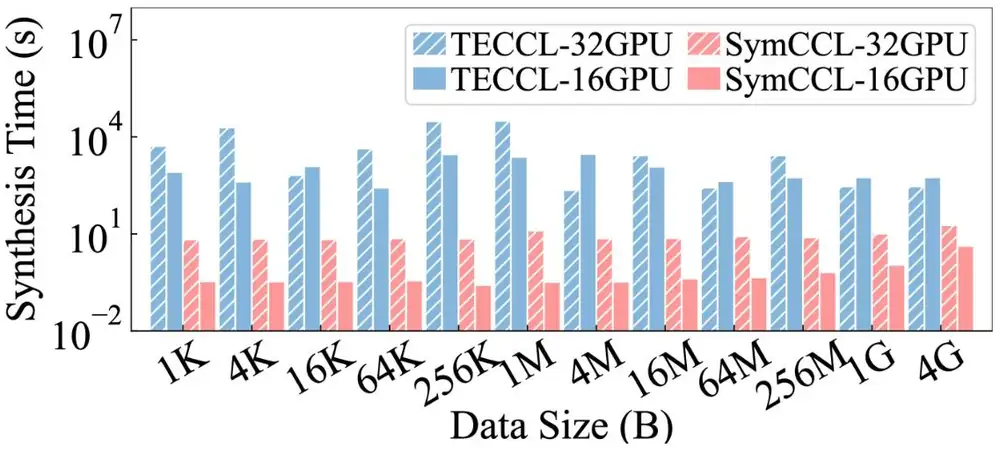
Figure 16(a) of the SyCCL paper: log-scale bars of synthesis time for TE-CCL and SymCCL at 16 and 32 GPUs, AllGather, data sizes 1 KB to 4 GB. — Figure 16(a) of the paper, measured run times: AllGather synthesis time on the 16- and 32-GPU A100 topology, 1 KB to 4 GB, log scale. Blue is TE-CCL, red is SyCCL (legend: SymCCL, an earlier name).論文的 Figure 16(a)，實測執行時間：16 與 32 GPU 的 A100 拓樸上 AllGather 的合成時間，1 KB 到 4 GB，對數座標。藍色是 TE-CCL，紅色是 SyCCL（圖例用舊名 SymCCL）。Screenshot of Cao et al., SIGCOMM 2025, Figure 16(a) (author PDF, p. 11).

At 512 GPUs almost all of the 37 minutes goes to the TE-CCL MILPs inside the groups; sketch search takes under a second. On a scaled H800 topology, pruning rules one and two cut synthesis time by 20.8–48.1%, and capping AllToAll sketches at 3 stages instead of 10 saved 95–97%.

在 512 GPU 時，37 分鐘幾乎全花在群組內的 TE-CCL MILP；sketch 搜尋不到一秒。在縮小的 H800 拓樸上，剪枝規則一與二把合成時間減少 20.8–48.1%，把 AllToAll 的 sketch 限制在 3 個階段而非 10 個，省下 95–97%。

End to end, the testbed trained GPT3-6.7B and Llama3-8B with data parallelism (distributed optimizer) or tensor parallelism. Iteration time in milliseconds (Table 6):

端到端方面，測試平台以資料平行（分散式最佳化器）或張量平行訓練 GPT3-6.7B 與 Llama3-8B。迭代時間，單位毫秒（Table 6）：

Model, parallelism模型、平行方式	NCCL	TE-CCL	SyCCL	SyCCL saves vs NCCL / TE-CCLSyCCL 相對 NCCL / TE-CCL 節省
GPT3-6.7B DP16	672.4	653.0	630.0	6.3% / 3.5%
GPT3-6.7B TP16	200.0	197.7	192.5	3.8% / 2.6%
GPT3-6.7B TP32	219.4	216.5	209.7	4.4% / 3.1%
Llama3-8B DP16	1,195.4	1,153.8	1,135.4	5.0% / 1.6%
Llama3-8B TP16	433.9	422.2	412.6	4.9% / 2.3%
Llama3-8B TP32	854.9	887.4	851.5	0.4% / 4.0%

Figure 4 plots the savings. In the last row TE-CCL's schedule was 3.8% slower than NCCL. Collective gains of up to 108% become iteration gains of 0.4–6.3%, because a collective fills only part of an iteration and some of it overlaps compute (Section 4.7).

圖 4 畫出節省的比例。在最後一列，TE-CCL 的排程比 NCCL 慢 3.8%。集體操作最多 108% 的增益，到了迭代只剩 0.4–6.3%，因為集體操作只占迭代的一部分，其中一些還與計算重疊（第 4.7 節）。

Figure 4. Table 6 as iteration time saved against NCCL,

(T_{\text{NCCL}} - T)/T_{\text{NCCL}}

, on the 32-GPU testbed (measured). SyCCL saves 0.4–6.3%; TE-CCL saves less, and in Llama3-8B TP32 it is slower than NCCL.圖 4。把 Table 6 畫成相對 NCCL 節省的迭代時間

(T_{\text{NCCL}} - T)/T_{\text{NCCL}}

，32 GPU 測試平台（實測）。SyCCL 節省 0.4–6.3%；TE-CCL 節省得較少，在 Llama3-8B TP32 甚至比 NCCL 慢。Drawn for this primer from Cao et al., SIGCOMM 2025, Table 6.

6. Limits and open questions6. 限制與未解的問題

The paper's own limits (§8): no optimality guarantee, since each MILP trades accuracy for time, pruning may drop a better sketch, and the $\alpha$ – $\beta$ model ignores congestion control and jitter; MoE AllToAllv breaks the symmetry; heterogeneous clusters reduce the benefit; regeneration after network changes works only when they are rare. A careful reader should add:

論文自己列出的限制（§8）：沒有最佳性保證，因為每個 MILP 都以準確度換時間、剪枝可能丟掉更好的 sketch，而且 $\alpha$ – $\beta$ 模型忽略壅塞控制與抖動；MoE 的 AllToAllv 會破壞對稱；異質叢集會降低效益；網路改變後重新產生排程，只在改變很少時可行。細心的讀者還應該補上：

Evidence. Hardware results stop at 32 GPUs; everything larger is simulated. TACCL is not a baseline.證據。硬體結果止於 32 顆 GPU；更大的規模都是模擬。TACCL 不在基準之列。
Symmetry is fragile. One failed NIC makes groups unequal, and 37 minutes at 512 GPUs cannot follow MoE traffic that changes every iteration.對稱很脆弱。一張故障的 NIC 就讓群組不再相同，而 512 GPU 時 37 分鐘的合成跟不上每次迭代都在變的 MoE 流量。
Consistency is assumed. The second pruning rule is an expectation; a later paper, OptCCL (SIGCOMM 2026), argues that it can lose optimality.一致性只是假設。第二條剪枝規則是一種預期；之後的 OptCCL（SIGCOMM 2026）主張它可能失去最佳性。
Loose ends. A800 or A100; $E_2$ is 0.5 in the setup but 0.2 is called appropriate in §7.4; Table 5 differs slightly from the ranges in the text.未對齊之處。A800 還是 A100；設定中 $E_2$ 是 0.5，§7.4 卻說 0.2 才恰當；Table 5 與正文中的範圍略有出入。

7. How it connects7. 與其他內容的關聯

TE-CCL (previous digest): SyCCL keeps its MILP and epochs but applies them inside groups.TE-CCL（上一篇導讀）：SyCCL 保留它的 MILP 與 epoch，但只用在群組內部。
Deep dive, sections 4, 7 and 8: the hierarchical all-reduce is one hand-made two-dimension sketch; overlap explains why iteration gains are small; bus bandwidth is the metric.第 4 章第 4、7、8 節：階層式 all-reduce 是一個人工設計的二維 sketch；重疊解釋了為何迭代增益很小；匯流排頻寬是這裡的指標。
Theseus lets a running job switch to new schedules when conditions change.Theseus 讓執行中的任務在條件改變時切換到新排程。
Guided readings: Rail-only and Alibaba HPN build the rail-optimized fabrics whose rails are SyCCL's dimension 1.論文導讀：Rail-only 與 Alibaba HPN 建造的 rail 最佳化網路，其 rail 就是 SyCCL 的維度 1。

Key numbers關鍵數字

Number	數字	Meaning
10.6%	Bandwidth NCCL's ring wastes on H800 (analysis with production parameters)	NCCL 環在 H800 上浪費的頻寬（使用生產參數的分析）
0.8 s vs 1,193 s	Mean synthesis, SyCCL vs TE-CCL, 16-GPU AllGather	平均合成時間，SyCCL 對 TE-CCL，16 GPU AllGather
915× – 17,286×	Synthesis speed-up of means, 16–64 GPUs	16–64 GPU 平均合成時間的加速
2,246 s ≈ 37 min	Mean synthesis at 512 GPUs; TE-CCL timed out	512 GPU 的平均合成時間；TE-CCL 逾時
+17% to +108%	Bus bandwidth over NCCL, 16-GPU AllGather above 1 MB (testbed)	16 GPU、1 MB 以上的 AllGather，匯流排頻寬相對 NCCL（測試平台）
0.4% – 6.3%	Iteration time saved against NCCL (testbed)	相對 NCCL 節省的迭代時間（測試平台）
887.4 vs 854.9 ms	TE-CCL slower than NCCL, Llama3-8B TP32	Llama3-8B TP32 中 TE-CCL 比 NCCL 慢

Terms used on this page本頁用到的術語

Dimension: One kind of GPU-to-GPU connection, such as NVSwitch or a rail's leaf switch.; 一種 GPU 之間的連線，例如 NVSwitch 或某條 rail 的 leaf 交換器。
Group: The GPUs joined directly in one dimension; isomorphic groups have identical internal wiring.; 在某個維度中直接相連的 GPU；同構的群組內部接線完全相同。
Sketch: A staged plan of sub-demands, each confined to one group of one dimension.; 由多個階段組成的子需求計畫，每個子需求限於某個維度的單一群組。
Sub-demand: A set of sources sending to a set of receivers inside one group.; 一組來源在單一群組內送給一組接收者。
Workload ratio: The data a plan puts on each dimension, matched to that dimension's share of bandwidth.; 一份計畫放在各維度上的資料量，要與該維度的頻寬占比相符。