Sharing the cluster: isolation, placement and spare capacity共用叢集:隔離、擺放與備用容量
Learn why a training cluster runs many jobs at once, how jobs disturb one another on a shared network, why placement is the strongest network lever, how allocation units fragment a cluster, and how operators keep a shared network healthy.了解為何一個訓練叢集同時跑許多任務、任務如何在共用的網路上互相干擾、為何擺放是最強的網路槓桿、配置單位如何讓叢集碎片化,以及營運者如何讓共用的網路保持健康。
This chapter builds on Chapters 3, 6, 7, 8, 10. These earlier terms appear most often below; each chip links to its definition.
New terms in this chapter (4)本章新名詞(4)
Each term is defined in the text where it first appears; the link jumps there. Terms from earlier chapters are listed under "Before you start".
每個名詞都在它第一次出現的段落中定義,點連結可跳過去。前面各章的名詞列在「開始之前」。
- Fragmentation碎片化 Free GPUs that exist but not in a shape a job can use without crossing racks or pods. 空閒 GPU 存在,但其形狀無法讓工作不跨機櫃或 pod 就使用。
- Isolation, contention隔離、爭用 Keeping one job's traffic from slowing another's; contention is two jobs wanting the same link. 避免一個工作的流量拖慢另一個;爭用是兩個工作想用同一條鏈路。
- Multi-tenancy, tenant多租戶、租戶 Several jobs or customers sharing one cluster and its network. 多個工作或客戶共用一個叢集及其網路。
- Placement, scheduler放置、排程器 Choosing which GPUs a job gets and which rank runs where; it decides which links the traffic crosses. 決定工作拿到哪些 GPU、各 rank 放在哪裡;它決定流量經過哪些鏈路。
11.1Why clusters are shared, and what sharing breaks叢集為何共用,以及共用會破壞什麼
A cluster is sized for the largest job it will ever run, but it runs that job rarely. HPN's Figure 6 says that 96.3% of Alibaba's LLM training jobs use fewer than 1,000 GPUs, on a pod built for 15,000. So the normal state of a cluster is tens of jobs of different sizes, starting and finishing at different times, and the scheduler must pack them. Two things go wrong when it does. Fragmentation means that free GPUs exist but not in a shape a job can use without crossing racks or segments. Queueing means that a job waits for a shape to become free. Both have a network cost, because a scheduler under pressure accepts a placement that spreads a job out.
叢集依它將跑過的最大任務來定規模,但很少真的跑那個任務。HPN 的 Figure 6 說,阿里 96.3% 的 LLM 訓練任務使用少於 1,000 顆 GPU,而 pod 是為 15,000 顆建的。所以叢集的常態是數十個大小不同、起訖時間不同的任務,排程器必須把它們裝進去。這麼做時會出兩種問題。碎片化指的是有空閒的 GPU,卻不是任務能在不跨機櫃或 segment 的情況下使用的形狀。排隊指的是任務等待某個形狀空出來。兩者都有網路代價,因為壓力下的排程器會接受把任務攤開的配置。
Work one example on an HPN segment: 128 hosts of 8 GPUs, 1,024 GPUs in all. Each host connects to all 8 ToR pairs, one pair per rail, so a job usually takes whole hosts. Job A takes 640 GPUs, 80 hosts. Job B takes 256, 32 hosts. 16 hosts are free. A new job of 256 GPUs cannot fit. It either waits until A or B finishes, or it takes 128 GPUs here and 128 in another segment, and from then on every one of its collectives crosses the aggregation layer. Figure 11.1 draws the example.
在一個 HPN segment 上算一個例子:128 台主機、每台 8 顆 GPU,共 1,024 顆。每台主機都連到全部 8 對 ToR,每個 rail 一對,所以任務通常以整台主機為單位。任務 A 拿 640 顆,80 台主機。任務 B 拿 256 顆,32 台主機。剩下 16 台主機是空的。一個新的 256 顆 GPU 任務放不進去。它要嘛等 A 或 B 結束,要嘛在這裡拿 128 顆、到另一個 segment 拿 128 顆,從此它的每一次集體操作都跨越聚合層。圖 11.1 畫出這個例子。
What one job does to another一個任務對另一個任務的影響
Crux measured the network case: a GPT job that shared links with a BERT job took 11% longer per iteration, 1.70 s instead of 1.53 s on average (Figure 11.2).
Crux 量測了網路的情形:與 BERT 任務共用鏈路的 GPT 任務,每次迭代平均多花 11%,從 1.53 秒變成 1.70 秒(圖 11.2)。
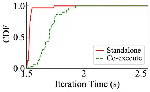
Once two jobs share switches, three mechanisms couple them. The first is hash collision. A training GPU has few flows, about 4 queue pairs per GPU for an AllReduce in Meta's measurement, so when job A's flow and job B's flow hash onto the same uplink, both run at half speed and every GPU waiting on either flow idles. HPN measured the cost directly: with four AllReduce jobs running at once on 512 GPUs, choosing disjoint paths on the host raised collective performance by up to 34.7%.
一旦兩個任務共用交換器,三種機制把它們耦合在一起。第一是雜湊碰撞。訓練 GPU 的流很少,Meta 量到 AllReduce 每顆 GPU 約 4 個 queue pair,所以當任務 A 的流與任務 B 的流被雜湊到同一條上行,兩者都只剩一半速度,等待任一條流的每顆 GPU 都在閒置。HPN 直接量出代價:512 顆 GPU 上同時跑四個 AllReduce 任務時,在主機端挑選不相交路徑讓集體通訊效能最多提升 34.7%。
The second is priority flow control (PFC). RoCE needs a lossless fabric, and PFC provides it by pausing an upstream port when a buffer fills. PFC pauses ports, not flows, so a pause caused by one job stops every job on that port. The DCQCN paper measured two consequences. In the parking-lot experiment, a sender with its own ingress port reached up to 20 Gb/s while three senders sharing one port split that port's share. In the victim flow experiment, a flow whose path shared no congested link with anyone fell from 20 Gb/s to 10 Gb/s because pause frames from an incast elsewhere cascaded through a switch it traversed, and to 4.5 Gb/s when two more incast senders joined. In a training pod, one job's reduce-scatter incast can pause the ring of a job that shares nothing with it except a switch.
第二是優先權流量控制(PFC)。RoCE 需要無損網路,PFC 在緩衝填滿時暫停上游埠來提供它。PFC 暫停的是埠而不是流,所以一個任務造成的暫停會停止該埠上的每一個任務。DCQCN 論文量到兩個後果。在停車場實驗中,擁有自己入口埠的發送端達到最高 20 Gb/s,共用一埠的三個發送端則分那個埠的份額。在受害者流實驗中,一條路徑與任何人都不共用壅塞鏈路的流,因為別處 incast 的暫停幀串聯穿過它經過的交換器,從 20 Gb/s 掉到 10 Gb/s,再有兩個 incast 發送端加入時掉到 4.5 Gb/s。在訓練 pod 裡,一個任務的 reduce-scatter incast 可以暫停另一個除了交換器之外與它毫無共用的任務的環。
The third is unequal cost. Alibaba's Crux (SIGCOMM 2024) measured that 36.3% of jobs in their cluster were at risk of contention, that is, of competing with another job for the same link, and proposed a rule: give the link to the job whose waiting GPUs are worth the most, because
第三是代價不對等。阿里的 Crux(SIGCOMM 2024)量到他們叢集中 36.3% 的任務有競爭(與另一個任務爭用同一條鏈路)的風險,並提出一條規則:把鏈路給等待中 GPU 價值最高的任務,因為
Figure 11.3 is the paper's own example.
圖 11.3 是論文自己的例子。
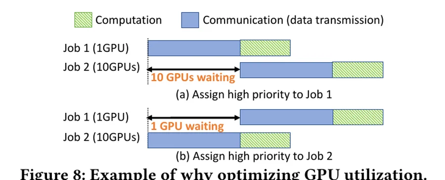
Panel 11.1 lets you apply the rule to two jobs that share one link.
面板 11.1 讓你把這條規則套用到共用一條鏈路的兩個任務。
Animation 11.1 plays the default case of Panel 11.1 in time, with both jobs' timelines under fair share and under Crux's priority.
動畫 11.1 把面板 11.1 的預設情況按時間播放,畫出兩個任務在平分鏈路與 Crux 優先權下的時間軸。
Isolation mechanisms and what they cost隔離機制與它們的代價
Isolation means that job A's traffic cannot change job B's step time. Four mechanisms exist, each at a different layer and price.
隔離指的是任務 A 的流量無法改變任務 B 的步時間。有四種機制,各在不同的層次、有不同的價格。
| Mechanism | 機制 | What it separates | 分開什麼 | What it does not fix, and its cost | 沒修好什麼,以及代價 | Where | 出處 |
|---|---|---|---|---|---|---|---|
| Lossless priority classes | 無損優先權類別 | Buffers and PFC pauses per class: a control or storage class cannot pause a data class | 每類別的緩衝與 PFC 暫停:控制或儲存類別不能暫停資料類別 | Links still shared, so collisions remain; each lossless class needs reserved headroom, so operators commonly run one or two | 鏈路仍共用,碰撞仍在;每個無損類別需要保留的 headroom,營運者通常只跑一到兩個 | Microsoft RoCE; Meta's high-priority CTS queue | Microsoft RoCE;Meta 的高優先權 CTS 佇列 |
| Per-tenant NICs on one host | 同一主機上每租戶專屬 NIC | Each tenant owns some of the 8 NICs and their ToR ports | 每個租戶擁有 8 張 NIC 中的一部分及其 ToR 埠 | No relaying through GPUs the tenant does not own, so rail-only's NVLink detour is forbidden; tier 2 must stay any-to-any | 不能透過不屬於租戶的 GPU 中繼,rail-only 的 NVLink 繞路被禁止;第二層必須維持任意對任意 | HPN §10, serverless use | HPN §10,serverless 用法 |
| Physical slice (air gap) | 實體切片(air gap) | Links and switches: two slices never share any | 鏈路與交換器:兩個切片永不共用 | Circuits reserved even when idle; shapes limited to ; re-wiring takes milliseconds | 電路閒置時也被保留;形狀限於 ;重新接線需要毫秒 | TPU v4 OCS slices | TPU v4 的 OCS 切片 |
| Rail- or segment-aware allocation | 依 rail 或 segment 感知的配置 | Keeps a job under one ToR set, so most traffic crosses one switch | 把任務留在一組 ToR 下,多數流量只跨一台交換器 | Holds only while the allocation holds; needs backup hosts; fragments the cluster | 只在配置成立時有效;需要備援主機;使叢集碎片化 | HPN segments; MegaScale ToR sets | HPN 的 segment;MegaScale 的 ToR 組 |
Two rows deserve a note. In HPN's serverless use, several tenants, customers renting GPUs, share one host and each owns some of its eight NICs; a tenant cannot relay traffic through a GPU it does not own, so the NVLink detour that rail-only topologies depend on is forbidden. That is one of the two reasons HPN kept an any-to-any aggregation layer instead of a rail-only one that could have held 120,000 GPUs per pod: multi-tenancy changed the topology. TPU v4 is the opposite extreme: every optical circuit belongs to one slice, so two slices never share a link or a switch, and this air gap is the only mechanism in the table that removes hash collisions, PFC coupling and buffer sharing at once. Its price is circuits that sit reserved while idle.
兩行值得補充。在 HPN 的 serverless 用法中,數個租戶(租用 GPU 的客戶)共享一台主機,各擁有八張 NIC 中的一部分;租戶不能透過不屬於自己的 GPU 中繼流量,所以 rail-only 拓樸所依賴的 NVLink 繞路被禁止。這是 HPN 保留任意對任意聚合層、而不採用每個 pod 可容納 120,000 顆 GPU 的 rail-only 的兩個理由之一:多租戶改變了拓樸。TPU v4 是另一個極端:每條光電路屬於一個切片,所以兩個切片永不共用鏈路或交換器,這個 air gap 是表中唯一能一次消除雜湊碰撞、PFC 耦合與緩衝共用的機制。代價是電路閒置時仍被保留。
11.2Placement: the strongest network lever擺放:最強的網路槓桿
A job does not have one traffic matrix. It has one traffic matrix per placement, the assignment of its ranks to particular GPUs. The bytes each dimension moves per step are fixed by the model and the parallelism; where those bytes go is fixed by where the ranks sit. HPN's Table 3 gives the per-step volumes for GPT-3 175B at , , : tensor parallelism moves 560 MB in all-reduce and all-gather, data parallelism 5.5 GB in all-reduce, and pipeline parallelism 6 MB in point-to-point sends. You can check the DP number:
一個任務沒有單一的流量矩陣。它每一種擺放(把它的 rank 分配到哪些 GPU)都有一個流量矩陣。每個維度每步搬動的位元組數由模型與平行化決定;這些位元組往哪裡去,由 rank 坐在哪裡決定。HPN 的 Table 3 給出 GPT-3 175B 在 、、 下每步的量:張量平行在 all-reduce 與 all-gather 中搬 560 MB,資料平行在 all-reduce 中搬 5.5 GB,管線平行在點對點傳送中搬 6 MB。DP 的數字可以驗算:
| Question問題 | Calculation算式 | Result結果 |
|---|---|---|
| Gradients of 175 billion parameters at 2 bytes each1,750 億參數、每個 2 位元組的梯度 | GB | |
| Shard per GPU, over the GPUs that hold one copy每顆 GPU 的分片,分給持有一份副本的 顆 GPU | GB | |
| Bytes through each GPU's NIC per step, ring all-reduce over , of the shard 的環狀 all-reduce 每步通過每顆 GPU NIC 的位元組,分片的 | GB |
So HPN's 5.5 GB is one GPU's gradient shard, and the ring moves about twice that, 11 GB, through each GPU's NIC every step.
所以 HPN 的 5.5 GB 就是一顆 GPU 的梯度分片,而環每步讓約兩倍的量、11 GB 通過每顆 GPU 的 NIC。
Now follow the bytes. In a ring, every GPU sends to one neighbor. If the neighbor is in the same server, the bytes ride NVLink at about 450 GB/s per direction and never touch the fabric. If it is in the same pod, they cross one or two switches at full rate. If it is in another pod, they cross the oversubscribed links: 1:7 at Meta, 15:1 at HPN. For any boundary, A ring whose ranks are ordered pod by pod crosses each pod boundary once; a ring whose ranks are scattered crosses on almost every hop. Figure 11.4 shows both cases.
現在跟著位元組走。在環中,每顆 GPU 送給一個鄰居。如果鄰居在同一台伺服器,位元組走每方向約 450 GB/s 的 NVLink,完全不碰網路。如果在同一個 pod 內,以全速跨一到兩台交換器。如果在另一個 pod,跨越超額認購的鏈路:Meta 是 1:7,HPN 是 15:1。對任何邊界,rank 依 pod 排列的環每個 pod 邊界只跨一次;rank 散落的環幾乎每一跳都跨。圖 11.4 畫出兩種情況。
Animation 11.2 moves the chunks of one ring all-gather on both placements of Figure 11.4.
動畫 11.2 在圖 11.4 的兩種配置上,逐步移動一次環狀 all-gather 的 chunk。
Three schedulers, one rule三個排程器,一條規則
Meta's scheduler learns where every server sits in the topology and assigns the ranks of a job so that the cut between AI Zones carries as little traffic as possible. In graph terms, the ranks are nodes, the per-step bytes between them are edge weights, and the scheduler looks for the partition into zones with the minimum cut. Inside a zone the fabric is non-blocking, so what remains is path choice, and there Meta deployed centralized traffic engineering (TE), a controller that assigns a path to every flow and held link utilization near 80% where hashing swung between 40% and 90%. Meta did not deploy TE across zones, because a controller reacting to every failure and job change at data-center scale was judged not worth the gain.
Meta 的排程器學習每台伺服器在拓樸中的位置,並指派任務的 rank,使 AI Zone 之間的切割承載最少的流量。用圖論的話說,rank 是節點、它們之間每步的位元組數是邊權重,排程器尋找跨 zone 的最小割分割。zone 內部網路是非阻塞的,剩下的是路徑選擇,Meta 在那裡部署了集中式流量工程(TE):一個為每條流指派路徑的控制器,在雜湊讓使用率於 40% 到 90% 之間擺盪時把它維持在 80% 附近。Meta 沒有跨 zone 部署 TE,因為在資料中心規模下對每次故障與任務變動做反應的控制器被判定不值得那點收益。
Llama 3 shows the rule applied to one run. The parallel dimensions are ordered [TP, CP, PP, DP], innermost first, and the innermost dimension gets the fastest link. Take Table 4, row 2: 16,384 GPUs, , , , . A TP group is one server on NVLink; a block is GPUs, 8 racks of 16, placed inside one 3,072-GPU pod. A pod holds 24 such blocks, so 128 blocks fill five pods and part of a sixth, each DP group of 128 spans 6 pods, and only FSDP's reduce-scatter and all-gather cross the 1:7 links; the paper allows this because FSDP traffic can be prefetched. Estimate the cost, with 50 GB/s per GPU and a pod-ordered ring in which only the boundary hops cross:
Llama 3 展示這條規則在一次運行上的應用。平行維度依 [TP, CP, PP, DP] 排序、最內層在前,最內層得到最快的鏈路。取 Table 4 第二行:16,384 顆 GPU、、、、。TP 群組就是一台走 NVLink 的伺服器;一個 區塊是 顆 GPU,即 8 個 16 顆的機櫃,放在一個 3,072 顆 GPU 的 pod 內。一個 pod 容納 24 個這樣的區塊,所以 128 個區塊填滿五個 pod 再加第六個的一部分,每個 128 的 DP 群組橫跨 6 個 pod,只有 FSDP 的 reduce-scatter 與 all-gather 跨越 1:7 鏈路;論文允許這樣是因為 FSDP 流量可以預先抓取。估算代價,以每顆 GPU 50 GB/s、依 pod 排列且只有邊界跳數跨越的環計:
| Question問題 | Calculation算式 | Result結果 |
|---|---|---|
| A block's gradient shard per GPU (405B parameters, 2 bytes, 128 GPUs)一個區塊每顆 GPU 的梯度分片(4,050 億參數、2 位元組、128 顆 GPU) | GB | |
| Reduce-scatter plus all-gather, per GPU per stepreduce-scatter 加 all-gather,每顆 GPU 每步 | GB | |
| Ring time at 50 GB/s, whether or not it crosses pods50 GB/s 下的環時間,不論是否跨 pod | s | |
| Bytes each pod sends over its uplinks per step (128 groups)每個 pod 每步透過上行送出的位元組(128 個群組) | TB | |
| A pod's uplink at 1:71:7 下一個 pod 的上行 | TB/s | |
| Time the uplink is busy上行忙碌的時間 | s | |
| GPUs per pod that may have a ring neighbor outside before the uplink saturates上行飽和之前,一個 pod 內可有環鄰居在 pod 外的 GPU 數 | ||
| Ring share of a 6 s step (16M-token batch at 400 TFLOP/s per GPU)環占 6 s 一步的比例(16M token 的批次、每顆 GPU 400 TFLOP/s) |
Each pod sends about 3.2 TB per step, and its uplinks are busy for about 0.15 s, less than the 0.25 s the ring takes anyway. The oversubscribed links are not the bottleneck; they would become one only if more than about 440 GPUs in a pod had a ring neighbor outside it. Against the whole step the ring is 4%, mostly prefetched. Table 4 agrees: doubling from 8K to 16K GPUs cost 2 MFU points, 43% to 41%.
每個 pod 每步送出約 3.2 TB,上行忙碌約 0.15 s,少於環本來就需要的 0.25 s。超額認購的鏈路不是瓶頸;只有當一個 pod 內超過約 440 顆 GPU 的環鄰居在 pod 外時,它才會成為瓶頸。對比整個步時間,環占 4%,且大多被預先抓取。Table 4 吻合:從 8K 加倍到 16K 顆 GPU 損失 2 個 MFU 百分點,43% 到 41%。
HPN draws the line one dimension lower. Its scheduler keeps TP and DP inside a pod and lets only pipeline traffic cross the core, because 6 MB per step is the smallest volume and point-to-point sends are the least bandwidth-sensitive. That is what makes a 15:1 core acceptable, and 64 backup GPUs per segment keep a job in place when a host fails. MegaScale states the same rule at rack scale: up to 64 servers share one set of eight ToRs, and the scheduler places communication-heavy ranks under the same ToR set so that most traffic crosses one switch. Figure 11.5 puts the Llama 3 and HPN layouts side by side.
HPN 把線畫低一個維度。它的排程器把 TP 與 DP 留在 pod 內,只讓管線流量跨越核心層,因為每步 6 MB 是最小的量,而點對點傳送對頻寬最不敏感。這就是 15:1 的核心層可以接受的原因,而每個 segment 64 顆備用 GPU 讓主機故障時任務留在原位。MegaScale 在機櫃尺度陳述同樣的規則:最多 64 台伺服器共用一組八台 ToR,排程器把通訊密集的 rank 放在同一組 ToR 下,讓多數流量只跨一台交換器。圖 11.5 把 Llama 3 與 HPN 的配置並排。
What a wrong placement costs擺錯的代價
HPN's headline experiment is the clearest measurement of placement in the literature, even though the paper presents it as a topology result. A production job of more than 2,300 GPUs ran on the old network, DCN+, spread over 19 segments. On HPN it fit in 3. Cross-segment traffic fell 37% on average and end-to-end training throughput rose 14.9%. Part of the gain is dual-plane removing hash polarization; the paper's ablation attributes up to 71.6% of the cross-segment gain to it. The rest is that fewer bytes crossed in the first place. The panel below lets you build the Llama 3 layout and then break it.
HPN 的主要實驗是文獻中對配置最清楚的量測,儘管論文把它當作拓樸結果呈現。一個超過 2,300 顆 GPU 的生產任務在舊網路 DCN+ 上橫跨 19 個 segment。在 HPN 上只需 3 個。跨 segment 流量平均減少 37%,端到端訓練吞吐提高 14.9%。部分增益來自 dual-plane 消除 hash polarization;論文的消融把跨 segment 增益中最多 71.6% 歸於它。其餘是一開始就少了跨越的位元組。下面的面板讓你先建出 Llama 3 的配置,再把它弄壞。
Keep the Llama 3 defaults and switch the placement to random. Read the crossing hops and the extra step time. Then set oversubscription to 15:1 and placement to sequential: this is HPN's rule, with only PP crossing. Why does the topology-aware layout show no extra time even at 15:1, and what, other than bytes, made Llama 3 put DP rather than PP across pods?
保留 Llama 3 的預設值,把配置切到隨機。讀跨越跳數與額外步時間。然後把超額認購設成 15:1、配置設成順序填入:這是 HPN 的規則,只有 PP 跨越。為什麼拓樸感知的配置即使在 15:1 也沒有額外時間?除了位元組之外,是什麼讓 Llama 3 把 DP 而不是 PP 放到跨 pod?
11.3Job shapes, fragmentation and spare capacity任務形狀、碎片化與備用容量
A scheduler allocates in units, and the unit decides the fragmentation. TPU v4's unit is a cube of 64 chips, and a slice may be any shape: a 192-chip job gets , so sizes need not be powers of two. More important, the shape can match the parallelism. A pipeline-parallel job with many stages asks for a 512-chip cigar, which gives the pipeline a long axis; a job that wants bisection bandwidth asks for . Table 3 of the paper shows that choosing topology and hyperparameters per job gained 1.2× to 2.3×: 2.3× between a novice's choice and the best for an LLM on 512 chips, 1.2× over an expert's choice for GPT-3 pre-training.
排程器以單位分配,單位決定碎片化。TPU v4 的單位是 64 顆晶片的 cube,切片可以是任何 的形狀:192 顆晶片的任務拿到 ,所以大小不必是二的冪。更重要的是,形狀可以符合平行化。階段很多的管線平行任務要一個 512 顆晶片、 的雪茄,給管線一條長軸;想要對分頻寬的任務要 。論文的 Table 3 顯示依任務選擇拓樸與超參數帶來 1.2 到 2.3 倍的增益:512 顆晶片上訓練 LLM,新手的選擇與最佳選擇相差 2.3 倍;GPT-3 預訓練比專家的選擇好 1.2 倍。
Panel 11.3 lets you build a slice and compare the two 512-chip shapes.
面板 11.3 讓你組出一個切片,並比較兩種 512 顆晶片的形狀。
GPU clusters allocate in racks and ToR sets: a Meta rack holds 16 GPUs under one ToR, an HPN ToR pair serves 128 GPUs, a MegaScale ToR set serves up to 64 servers. The unit is coarse because the fabric is wired for it. Rail-optimized wiring assumes that GPU of every host under a ToR set belongs to the same job, and path pinning assumes that every downlink of a rack is in use. Meta's path-pinning stage shows what happens when a rack is half allocated: one of its two hosts used the uplinks and the other did not, so some uplinks idled while others overloaded, and training slowed by more than 30%. Figure 11.6 sketches this case.
GPU 叢集以機櫃與 ToR 組分配:Meta 的一個機櫃在一台 ToR 下有 16 顆 GPU,HPN 的一對 ToR 服務 128 顆 GPU,MegaScale 的一組 ToR 服務最多 64 台伺服器。單位粗是因為網路就是為它接線的。rail-optimized 接線假設一組 ToR 下每台主機的 GPU 都屬於同一個任務,路徑固定假設機櫃的每條下行都在使用中。Meta 的路徑固定階段顯示機櫃分配一半時會怎樣:兩台主機中只有一台在用上行、另一台沒有,所以某些上行閒置、另一些過載,訓練慢了超過 30%。圖 11.6 畫出這個情況。
Every operator keeps spare capacity, and the amount is a policy. HPN reserves 8 of each ToR's 136 host-facing ports as backup, so a segment has 1,024 active GPUs plus 64 spare, 6.25%; a failed host is replaced inside the segment and the job keeps its placement. Meta's final design gives each rack switch 1:1.125 uplink bandwidth, 12.5% more than the downlinks need, chosen so that two failed uplinks do not slow a job; the 1:2 ratio used earlier worked but doubled the cost of the network. The formula behind every row of the table is the same: rounded up to the allocation unit. Figure 11.7 draws the two policies.
每個營運者都保留備用容量,保留多少是政策。HPN 把每台 ToR 136 個面向主機的埠中的 8 個保留為備援,所以一個 segment 有 1,024 顆使用中 GPU 加 64 顆備用,即 6.25%;故障主機在 segment 內被替換,任務保持其配置。Meta 的最終設計給每台機櫃交換器 1:1.125 的上行頻寬,比下行所需多 12.5%,選擇這個值是為了讓兩條上行故障不會拖慢任務;早先用的 1:2 有效,但讓網路成本加倍。表中每一行背後的公式相同:再向上取到配置單位。圖 11.7 畫出這兩種政策。
| Operator | 營運者 | Allocation unit | 配置單位 | Spare policy | 備用政策 | Measured consequence | 量到的後果 |
|---|---|---|---|---|---|---|---|
| Alibaba HPN | Segment: 1,024 GPUs under 16 ToRs; 15 segments per pod | segment:16 台 ToR 下 1,024 顆 GPU;每 pod 15 個 segment | 64 backup GPUs per segment; only PP crosses pods | 每個 segment 64 顆備用 GPU;只有 PP 跨 pod | 19 → 3 segments: +14.9% throughput, −37% cross-segment traffic | 19 → 3 個 segment:吞吐 +14.9%,跨 segment 流量 −37% | |
| Meta / Llama 3 | Rack of 16 GPUs; AI Zone; pod of 3,072 GPUs | 16 顆 GPU 的機櫃;AI Zone;3,072 顆 GPU 的 pod | 1:1.125 rack-switch uplinks; minimum-cut placement | 機櫃交換器上行 1:1.125;最小割配置 | Partly allocated racks under path pinning: >30% slower | 路徑固定下機櫃部分分配:慢 >30% | |
| ByteDance MegaScale | ToR set: up to 64 servers on 8 ToRs | ToR 組:8 台 ToR 上最多 64 台伺服器 | Standby node pool, automatic swap | 備用節點池,自動換機 | >100 restarts in weeks; effective training time >90% | 數週內重啟 >100 次;有效訓練時間 >90% | |
| Google TPU v4 | Cube of 64 chips; slice of | 64 顆晶片的 cube; 的切片 | OCS rewires around failed cubes | OCS 繞過故障 cube | 75% goodput for a quarter-machine slice at 99.0–99.5% availability | 四分之一機器的切片在 99.0–99.5% 可用性下 75% goodput |
Priorities and preemption are the part of this topic with the least published evidence. Crux's rule, serve the job with the most GPU-time at stake, is a priority on the link. Schedulers can also apply priority to the GPUs: a large job may preempt small ones to obtain a contiguous shape, at the cost of the preempted jobs' progress since their last checkpoint, which HPN says comes every two to four hours. How often operators choose preemption over waiting is not reported in these papers, so treat the trade-off as a policy question rather than a settled result.
優先權與搶占是本主題中已發表證據最少的部分。Crux 的規則——服務 GPU 時間損失最大的任務——是鏈路上的優先權。排程器也可以對 GPU 施加優先權:大任務可以搶占小任務以取得連續的形狀,代價是被搶占任務自上次檢查點以來的進度;HPN 說檢查點每二到四小時一次。這些論文沒有報告營運者多常選擇搶占而非等待,所以把這個權衡當作政策問題,而不是已有定論的結果。
Animation 11.3 plays fragmentation in two segments and the three ways out: wait, split, or move a running job.
動畫 11.3 在兩個 segment 中演出碎片化,以及三條出路:等待、拆開,或搬動正在跑的任務。
11.4Operating a shared network營運一個共用的網路
A shared fabric is never finished: jobs come and go, hosts fail, switches are upgraded, and a new GPU generation arrives every two years. The operators converge on three practices: per-job telemetry that attributes a symptom to a tenant, verification of the physical build before any end-to-end test, and change management that assumes upgrades break things.
共享的網路永遠沒有完工的一天:任務來來去去、主機故障、交換器升級,每兩年又有新一代 GPU 到來。營運者在三個做法上趨於一致:把症狀歸到租戶的逐任務遙測、任何端到端測試之前先驗證實體建置、以及假設升級會弄壞東西的變更管理。
Telemetry that names the job能指出是哪個任務的遙測
| Signal | 訊號 | Threshold or form | 門檻或形式 | What it catches | 抓到什麼 | Source | 出處 |
|---|---|---|---|---|---|---|---|
| RDMA traffic counters in the node heartbeat | 節點心跳中的 RDMA 流量計數器 | Sudden drop alerts; full stop triggers recovery | 突然下降發警報;完全停止觸發恢復 | A hung rank or a flapping NIC, attributed to the job | 卡住的 rank 或抖動的 NIC,歸到該任務 | MegaScale §4 | |
| PFC watchdog | PFC watchdog | 200 ms | A port paused too long, which names the paused tenant | 暫停過久的埠,指出被暫停的租戶 | Meta RoCE §6; Microsoft used 100 and 200 ms | Meta RoCE §6;Microsoft 用 100 與 200 ms | |
| Buffer alarm | 緩衝警報 | 80% | A spine buffer about to pause or drop | 即將暫停或丟包的 spine 緩衝 | Meta RoCE §6 | ||
| Out-of-sequence packets, ACK timeouts, link flaps | 亂序封包、ACK 逾時、鏈路抖動 | NIC counters | NIC 計數器 | Loss, reordering, marginal links | 丟包、亂序、邊緣狀態的鏈路 | Meta RoCE §6 | |
| CUDA-event timing per rank | 逐 rank 的 CUDA 事件計時 | Heat map of step times | 步時間的熱圖 | The 0.5% of machines slow enough to pace the job | 慢到決定任務節奏的那 0.5% 機器 | MegaScale §5 | |
| INT probes | INT 探測封包 | Switch and port ID at each hop vs. blueprint | 每跳的交換器與埠 ID 對照藍圖 | Miswired rails and planes, before any end-to-end test | rail 與 plane 接錯,在任何端到端測試之前 | HPN §10 | |
| Reachability pings | 可達性 ping | Periodic, between all hosts | 所有主機之間定期執行 | Routes that silently disappeared | 悄悄消失的路由 | Meta RoCE §6 |
In a shared fabric every counter must be attributed. The scheduler knows which GPUs, and therefore which NICs and ToR ports, belong to each job, so NIC counters map to tenants, a PFC watchdog names the tenant being paused, and a buffer alarm names the switch about to drop or pause. The CUDA-event monitor catches the slow tenant rather than the slow link: removing the 0.5% of slow machines it found made MegaScale's peak MFU consistent from run to run. Monitoring is also what caught Meta's CTSW software upgrade that raised port-to-port latency and silently slowed training.
在共享網路中每個計數器都必須有歸屬。排程器知道哪些 GPU、因而哪些 NIC 與 ToR 埠屬於每個任務,所以 NIC 計數器對應到租戶,PFC watchdog 指出被暫停的租戶,緩衝警報則指出即將丟包或暫停的交換器。CUDA 事件監控器抓的是慢的租戶而不是慢的鏈路:移除它找到的 0.5% 慢機器後,MegaScale 的峰值 MFU 在各次運行間變得一致。也是監控抓到了 Meta 那次提高埠對埠延遲、悄悄拖慢訓練的 CTSW 軟體升級。
Panel 11.4 shows why a small share of slow machines paces almost every large job, and how many spare machines it takes to swap them out.
面板 11.4 說明為什麼一小部分慢機器幾乎決定每個大任務的節奏,以及要多少備用機才能把它們換掉。
Animation 11.4 shows one slow machine pacing a synchronous job, and a spare that replaces it.
動畫 11.4 呈現一台慢機器如何拖慢同步任務,以及備用機如何替換它。
Verify the wiring, then stage the change先驗證接線,再分階段改動
HPN's rail-optimized plus dual-plane design means thousands of cables with exact required endpoints, and on-site staff made many mistakes in the early builds. The team now sends in-band network telemetry (INT) probes that record the switch ID and port ID at every hop and compares them against the blueprint before any end-to-end test. A miswired rail does not fail; it silently turns a one-switch path into a three-switch path, a symptom a shared fabric hides among other jobs' noise. Figure 11.8 shows one miswired cable.
HPN 的 rail-optimized 加 dual-plane 設計表示數千條線纜都有精確要求的兩端,早期建置時現場人員犯了很多錯。團隊現在在任何端到端測試之前,先送出帶內網路遙測(INT)探測封包,記錄每一跳的交換器 ID 與埠 ID,並與藍圖比對。接錯的 rail 不會失效;它悄悄把一跳交換器的路徑變成三跳,是共享網路會藏在其他任務雜訊中的症狀。圖 11.8 畫出一條接錯的線。
Upgrades are the other hazard. HPN found that 70% of its ToR upgrades did not meet the assumption behind in-service software upgrade, that old and new versions differ only slightly; the non-stacked dual-ToR exists partly so that one ToR can be upgraded while the other carries the host at 6.25% lower throughput (Section 6.5). Microsoft's RoCE rollout was staged: lab, test clusters, PFC on ToRs only, then a podset, then the spine; even so, a buffer threshold changed from 1/16 to 1/64 on a new switch model propagated PFC to thousands of servers until it was reverted. The rule is to change one tier at a time, with the monitoring watching, and with a way back.
升級是另一個風險。HPN 發現 70% 的 ToR 升級不符合不中斷服務升級背後的假設——新舊版本只有微小差異;非堆疊式 dual-ToR 存在的部分原因,就是讓一台 ToR 升級時另一台以低 6.25% 的吞吐撐住主機(第 6.5 節)。Microsoft 的 RoCE 部署是分階段的:實驗室、測試叢集、只在 ToR 開 PFC、然後一個 podset、然後 spine;即便如此,新交換器型號上一個從 1/16 改到 1/64 的緩衝門檻仍把 PFC 擴散到數千台伺服器,直到被回退。規則是:一次只改一層,讓監控盯著,並留一條退路。
Capacity planning across generations跨世代的容量規劃
The last operating problem is that the cluster outlives its design point. HPN sized a pod to one building, 18 MW, about 15,000 GPUs, so that every fiber stays under 100 m and can use multi-mode transceivers at 70% lower cost; the next generation is planned around 102.4 Tb/s chips, and new buildings have had their power budgets raised to match. How many GPUs one job may span at full rate is fixed by the switch radix and the building, and revisited only when a chip generation changes. The arithmetic for a two-tier pod is short: which for HPN is ; ; and the oversubscription toward the core decides how much of the pod one job may really use. When a model class changes the traffic, as mixture-of-experts does with all-to-all between experts on different rails, the placement rule has to be rewritten first.
最後一個營運問題是叢集活得比它的設計點更久。HPN 把一個 pod 定在一棟樓、18 MW、約 15,000 顆 GPU,讓每條光纖都低於 100 m、可以用便宜 70% 的多模光模組;下一代圍繞 102.4 Tb/s 晶片規劃,新建築的電力預算也已相應提高。一個任務可以全速橫跨多少顆 GPU,由交換器埠數與建築決定,只在晶片世代改變時重新檢視。兩層 pod 的算術很短:HPN 是 ;而朝核心層的超額認購決定單一任務真正能用多少個 pod。當某類模型改變流量——像混合專家在不同 rail 上的專家之間帶來 all-to-all——配置規則得先重寫。
A training cluster is sized for its largest job but mostly runs many smaller ones: on HPN's pod, 96.3% of jobs use fewer than 1,000 GPUs. Jobs that share switches disturb one another through hash collisions, PFC pauses that cross job boundaries, and links shared unequally; Crux measured a GPT job 11% slower beside a BERT job. Placement is the strongest lever: the same job moves different bytes over the thin links depending on which GPUs it gets, and the three schedulers of this book all keep the heavy dimensions inside the full-bandwidth part of the network. Allocation units (racks, ToR pairs, TPU cubes) fragment a cluster, and every operator keeps spare hosts or uplinks. A shared network needs telemetry attributed to jobs, verified wiring and staged changes.
訓練叢集是依最大的任務設計的,但大部分時間跑的是許多較小的任務:在 HPN 的 pod 上,96.3% 的任務用不到 1,000 顆 GPU。共用交換器的任務會透過雜湊碰撞、跨越任務邊界的 PFC 暫停,以及不平均地共用鏈路而互相干擾;Crux 量到一個 GPT 任務在 BERT 任務旁慢了 11%。擺放是最強的槓桿:同一個任務拿到不同的 GPU,就會在細鏈路上搬不同的位元組;本書的三個排程器都把吃重的維度留在網路的滿頻寬部分。配置單位(機櫃、ToR 對、TPU cube)讓叢集碎片化,每個營運者都保留備用主機或上行。共用的網路需要歸屬到任務的遙測、經過驗證的接線,以及分階段的改動。
Chapter 12 asks how designers predict all of this before the hardware exists: simple models, simulators, and how to check them against measurements.
第 12 章探討設計者如何在硬體存在之前預測這一切:簡單的模型、模擬器,以及如何用量測檢驗它們。