The front end: data, checkpoints and control前端網路:資料、檢查點與控制
Learn why every training cluster has a second network, what travels on it (training data, checkpoints, management and monitoring), why checkpoints are the burst that sizes it, and how to size it.了解為何每個訓練叢集都有第二個網路、它承載什麼(訓練資料、檢查點、管理與監控)、為何檢查點是決定它規模的突發流量,以及如何決定它的大小。
This chapter builds on Chapters 1, 3, 5, 6, 7. These earlier terms appear most often below; each chip links to its definition.
New terms in this chapter (7)本章新名詞(7)
Each term is defined in the text where it first appears; the link jumps there. Terms from earlier chapters are listed under "Before you start".
每個名詞都在它第一次出現的段落中定義,點連結可跳過去。前面各章的名詞列在「開始之前」。
- Checkpoint檢查點(checkpoint) A saved copy of the training state (weights and optimizer state) from which a job can resume after a failure. 訓練狀態(權重與最佳化器狀態)的存檔,工作故障後可從此處恢復。
- Front-end and back-end networks前端網路與後端網路 The back end carries only GPU-to-GPU training traffic; the front end carries data, checkpoints, logs and management. 後端只承載 GPU 之間的訓練流量;前端承載資料、檢查點、日誌與管理流量。
- Distributed storage分散式儲存 Many storage servers that act as one file system or object store; its throughput is set by the number of servers. 許多儲存伺服器合為一個檔案系統或物件儲存;吞吐量由伺服器數決定。
- Two-stage checkpoint兩階段檢查點 Copy the state to host memory first (the GPUs pause for seconds), then write it to storage in the background. 先把狀態複製到主機記憶體(GPU 暫停數秒),再在背景寫入儲存。
- Erasure coding糾刪碼 Protecting data with k data fragments and m parity fragments instead of three full copies. 以 k 個資料片段加 m 個同位片段保護資料,而非存三份完整副本。
- Out-of-band management頻外管理 A separate slow network that reaches each server's management controller even when the host is down. 一條獨立的低速網路,即使主機當機也能連到每台伺服器的管理控制器。
- Telemetry遙測(telemetry) Counters and logs collected from hosts and switches to watch the network. 從主機與交換器收集的計數器與日誌,用來監看網路。
9.1Two networks, four kinds of traffic兩個網路、四種流量
The training traffic described so far is only one part. A job must also read its training data, write checkpoints (a full copy of the model, saved every few hours), send logs and metrics, and talk to the scheduler. This traffic has a different shape: it is TCP, it goes to storage servers, and a slow moment is annoying but not fatal. Mixing it with RDMA traffic would be dangerous. A burst of checkpoint writes could trigger PFC pauses that stall a collective.
前面描述的訓練流量只是其中一部分。一個任務還必須讀訓練資料、寫檢查點(模型的完整副本,每隔幾小時存一次)、送出日誌與指標,並與排程器溝通。這類流量形狀不同:它是 TCP、目的地是儲存伺服器,慢一下令人煩躁但不致命。把它和 RDMA 流量混在一起會很危險:一波檢查點寫入就可能觸發 PFC 暫停,讓集體通訊停擺。
So every design separates them. The back-end network (Meta's BE, Alibaba's "backend") carries only GPU-to-GPU RDMA. It is non-blocking inside a zone, lossless, and tuned for a few elephant flows. The front-end network (FE) carries everything else over the normal data center fabric. Each server has ports on both. Meta notes that the front-end must still have enough bandwidth to keep the GPUs fed with data; HPN builds the front end at 1:1 so it can also serve inference and mixed workloads.
所以每個設計都把它們分開。後端網路(Meta 的 BE、Alibaba 的「backend」)只承載 GPU 到 GPU 的 RDMA。它在區域內非阻塞、無損,並針對少數大象流調校。前端網路(FE)則透過一般的資料中心網路承載其他所有東西。每台伺服器在兩個網路上都有埠。Meta 指出前端仍必須有足夠頻寬,才能持續餵資料給 GPU;HPN 把前端做成 1:1,讓它也能服務推論與混合負載。
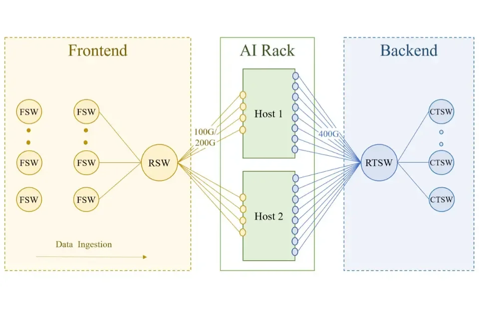
Mechanism. Every training host has ports on two fabrics. In Meta's Grand Teton server, eight RDMA NICs, one per GPU, each run at 400 Gb/s into the rack training switch (RTSW) of the back end; separate front-end NICs at 100 or 200 Gb/s connect to the ordinary rack switch (RSW), which leads through the fabric switches to the storage warehouse (Meta RoCE paper, Section 9.3). In HPN a host has nine NICs: NIC 0 serves the front end with two 200 Gb/s ports, and NICs 1–8 serve the back end, one per GPU, also at 2×200 Gb/s (HPN §3). The back end therefore offers 3.2 Tb/s per host and the front end 400 Gb/s. Figure 9.1 shows Meta's version of this split.
機制。每台訓練主機在兩個網路上都有埠。在 Meta 的 Grand Teton 伺服器裡,八張 RDMA NIC、每顆 GPU 一張,各以 400 Gb/s 接到後端的機櫃訓練交換器(RTSW);另有 100 或 200 Gb/s 的前端 NIC 接到一般的機櫃交換器(RSW),再經 fabric 交換器通往儲存倉庫(Meta RoCE 論文 §3)。在 HPN 裡一台主機有九張 NIC:NIC 0 以兩個 200 Gb/s 埠服務前端,NIC 1–8 服務後端、每顆 GPU 一張,同樣是 2×200 Gb/s(HPN §3)。因此後端每台主機有 3.2 Tb/s,前端有 400 Gb/s。圖 9.1 是 Meta 版本的這種分工。
The traffic that must stay off the GPU fabric. Four kinds of traffic travel on the front end, and HPN adds a fifth. Each has a different shape, and the shape decides how it is sized.
必須遠離 GPU 網路的流量。四種流量走在前端上,HPN 再加上第五種。每一種的形狀不同,而形狀決定了它怎麼定規模。
| Traffic | 流量 | Direction and shape | 方向與形狀 | What sets its size | 決定大小的因素 | If it is slow | 變慢的後果 |
|---|---|---|---|---|---|---|---|
| Dataset reads | 資料集讀取 | Storage → hosts; steady, prefetched | 儲存 → 主機;穩定,預先抓取 | GPUs wait for input; usually hidden | GPU 等待輸入;通常被遮住 | ||
| Checkpoint writes | 檢查點寫入 | Hosts → storage; one synchronized burst | 主機 → 儲存;一次同步的突發 | All GPUs stall until absorbed | 所有 GPU 停頓到吸收完 | ||
| Checkpoint reads | 檢查點讀取 | Storage → hosts; one burst per restart | 儲存 → 主機;每次重啟一次突發 | Shards without a copy on the fabric | 網路上沒有副本的分片 | Longer restart after every failure | 每次故障後重啟更久 |
| Logs and telemetry | 日誌與遙測 | Hosts → collectors; many small flows | 主機 → 收集器;許多小流 | Faults are found late | 故障發現得晚 | ||
| Control and management | 控制與管理 | Scheduler, heartbeats, images, PXE boot, SSH | 排程器、心跳、映像、PXE 開機、SSH | Small, except image pulls | 很小,拉取映像除外 | Slow start-up and recovery | 啟動與恢復變慢 |
| Inference (HPN) | 推論(HPN) | Clients ↔ hosts; request/response | 客戶端 ↔ 主機;請求/回應 | Requests per second; front-end heavy | 每秒請求數;以前端為主 | User-visible latency | 使用者看得見的延遲 |
Why they are separated. Meta gives the direct reason: a burst of checkpoint writes must never pause a collective, and the back end must be upgradable on its own schedule (Meta RoCE paper, Section 9.3). The mechanism is priority flow control: the back end is lossless, so a switch whose buffer fills sends a pause frame upstream, and the pause spreads hop by hop. A checkpoint is a many-to-one pattern, thousands of hosts writing to a few hundred storage servers at once. If those servers sat on the lossless fabric, the ports in front of them would fill and pause their upstream ports, and the pauses would reach the ports the collectives use: one slow storage server could stall an all-reduce on 16,000 GPUs. On a lossy TCP network the same incast drops packets, TCP backs off, and the checkpoint takes a little longer, the right failure mode for traffic nobody waits on microsecond by microsecond.
為什麼要分開。Meta 給出直接的理由:一波檢查點寫入永遠不能讓集體通訊暫停,而且後端必須能依自己的時程升級(Meta RoCE 論文 §3)。機制是優先權流量控制:後端是無損的,緩衝填滿的交換器向上游送出暫停幀,暫停一跳一跳地擴散。檢查點是多對一的模式,數千台主機同時寫向幾百台儲存伺服器。如果那些伺服器坐在無損網路上,它們前面的埠會填滿並暫停其上游埠,而暫停會一路傳到集體通訊使用的埠:一台慢的儲存伺服器就可能讓 16,000 顆 GPU 的 all-reduce 停擺。在有損的 TCP 網路上,同樣的 incast 只是丟包、TCP 退讓、檢查點多花一點時間,對沒有人以微秒為單位等待的流量來說,這才是正確的故障模式。
HPN's three reasons. The back end has eight times the front end's bandwidth, so HPN's authors considered putting storage there and rejected it for three reasons (HPN §8). Customers' datasets and container images live in other data centers, and an isolated back end cannot reach them without a proxy that copies every byte. Storage traffic injected into the back end as an experiment made training performance fluctuate: the PFC mechanism above, observed in practice. And storage servers consume ToR ports: a HPN ToR has 128 active host-facing 200G ports, and each one given to a storage server is one not given to a GPU. Storage stays on the front end, built non-blocking at 2×200 Gb/s per host so that the same machines can serve inference, whose traffic is front-end heavy. The HPN overview figure in Section 6.4 shows the result: the storage cluster sits inside HPN's front-end network.
HPN 的三個理由。後端有前端八倍的頻寬,所以 HPN 的作者曾考慮把儲存放到那裡,並基於三個理由拒絕(HPN §8)。客戶的資料集與容器映像放在其他資料中心,隔離的後端沒有一台逐位元組轉送的代理就無法到達它們。實驗中注入後端的儲存流量讓訓練效能出現波動:正是上面的 PFC 機制在實務中的樣子。而且儲存伺服器會消耗 ToR 埠:一台 HPN ToR 有 128 個使用中的面向主機 200G 埠,每一個給儲存伺服器的埠就是沒給 GPU 的埠。儲存留在前端,前端以每台主機 2×200 Gb/s 建成非阻塞,讓同樣的機器也能服務以前端流量為主的推論。第 6.4 節的 HPN 全貌圖顯示了結果:儲存叢集位在 HPN 的前端網路之內。
Meta's storage system is Tectonic, a distributed file system that spreads data over thousands of storage servers (Section 9.4). Panel 9.1 tests the case for the back end: does eight times more bandwidth per host (HPN) make a checkpoint faster?
Meta 的儲存系統是 Tectonic,一個把資料分散到數千台儲存伺服器上的分散式檔案系統(第 9.4 節)。面板 9.1 檢驗把儲存放上後端的理由:每台主機多八倍的頻寬(HPN),會讓檢查點變快嗎?
How the two networks differ. The table is the whole argument in one place. The back end is engineered never to drop a packet; the front end is engineered so that a drop is harmless.
兩個網路有何不同。下表把整個論證放在一處。後端的工程目標是永不丟包;前端的工程目標是丟包無害。
| Property | 性質 | Front end (FE) | 前端(FE) | Back end (BE) | 後端(BE) |
|---|---|---|---|---|---|
| Transport | 傳輸層 | TCP/IP; storage and HTTP protocols | TCP/IP;儲存與 HTTP 協定 | RoCEv2 (RDMA in UDP/IP) | RoCEv2(UDP/IP 中的 RDMA) |
| Loss | 丟包 | Lossy; drops are TCP's congestion signal | 有損;丟包是 TCP 的壅塞訊號 | Lossless; PFC pauses and deep buffers | 無損;PFC 暫停與深緩衝 |
| Oversubscription | 超額認購 | Several to one; HPN's 1:1 is the exception | 數比一;HPN 的 1:1 是例外 | 1:1 in a zone; 1:7 or 15:1 between pods | zone 內 1:1;pod 之間 1:7 或 15:1 |
| Sharing | 共用 | Shared with the data center | 與資料中心共用 | Dedicated to one training cluster | 專屬於一個訓練叢集 |
| Flows | 流 | Thousands of small flows; ECMP works | 數千條小流;ECMP 能用 | Tens of elephant flows per host; ECMP fails | 每台主機幾十條大象流;ECMP 失效 |
| Per host | 每台主機 | Meta 100/200G; HPN 2×200G | Meta 100/200G;HPN 2×200G | 8×400G (3.2 Tb/s) in both | 兩者都是 8×400G(3.2 Tb/s) |
| Cost of a slow second | 慢一秒的代價 | A later checkpoint or log line | 檢查點或日誌晚一點 | 16,000 GPUs idle for that second | 16,000 顆 GPU 閒置那一秒 |
9.2Dataset traffic: smaller than you think資料集流量:比你想的小
Mechanism. A language model consumes tokens. Each step processes one global batch, and the loader must deliver the next batch before the next step begins, so the front end must supply Llama 3 used a global batch of 16M tokens on 16,384 GPUs (Llama 3 Table 4). The step time is not published, but it can be derived from two facts: a dense transformer does about FLOP per token, and the cluster achieved about 400 TFLOP/s per GPU (Table 4, row 2). The arithmetic, one question per row:
機制。語言模型消耗 token。每一步處理一個全域批次,載入器必須在下一步開始前送到下一個批次,所以前端必須供應 Llama 3 在 16,384 顆 GPU 上使用 16M token 的全域批次(Llama 3 Table 4)。步時間沒有公布,但可以由兩個事實推導:稠密 transformer 每個 token 約做 FLOP,而叢集達到每顆 GPU 約 400 TFLOP/s(Table 4 第二行)。逐列計算如下:
| Question問題 | Calculation算式 | Result結果 |
|---|---|---|
| FLOP in one step of a 405B model over 16.8M tokens405B 模型對 16.8M 個 token 的一步 FLOP | FLOP | |
| Cluster rate: 16,384 GPUs at 400 TFLOP/s叢集速率:16,384 顆 GPU、每顆 400 TFLOP/s | FLOP/s | |
| Step time步時間 | sabout 6 seconds約 6 秒 | |
| Tokens consumed per second每秒消耗的 token 數 | 2.7 million tokens per second每秒約 270 萬個 token |
One step therefore took about 6 seconds, and the job consumed about 2.7 million tokens per second.
因此一步約 6 秒,任務每秒消耗約 270 萬個 token。
Bytes per token. Tokenized text is stored as integer ids: 2 bytes for a vocabulary up to 65,536, 4 bytes for Llama 3's 128K vocabulary in the usual integer formats. The dataset rate of the whole cluster is then MB/s, about 5 KB/s for each of 2,048 hosts. A 100G front-end NIC moves 12.5 GB/s, so dataset reads use about one millionth of it. The whole 15.6-trillion-token dataset is about 62 TB and is read once over the run.
每個 token 的位元組數。token 化後的文字以整數 id 儲存:詞彙表在 65,536 以內是 2 個位元組,Llama 3 的 128K 詞彙表在常見的整數格式下是 4 個位元組。整個叢集的資料集速率於是是 MB/s,2,048 台主機每台約 5 KB/s。一張 100G 前端 NIC 能搬 12.5 GB/s,所以資料集讀取只用了它的百萬分之一左右。整個 15.6 兆 token 的資料集約 62 TB,整段訓練只讀一遍。
Why it is small. A 405B model spends about FLOP on every token, and the token arrives as 4 bytes: about FLOP per byte. No network is a bottleneck at that ratio. What matters for text is the access pattern: shuffled reads across many shards, hidden by keeping batches in flight.
為什麼這麼小。405B 模型對每個 token 花約 FLOP,而 token 以 4 個位元組到達:每位元組約 FLOP。在這個比率下沒有任何網路會是瓶頸。對文字重要的是存取模式:打亂的讀取分散在許多分片上,靠讓批次在途來遮住延遲。
Panel 9.2 repeats this derivation for other models, clusters and token sizes.
面板 9.2 對其他模型、叢集與 token 大小重做這個推導。
Why it is large for images and video. The same formula with a different bytes-per-token changes the answer by orders of magnitude. A JPEG of a few hundred kilobytes that becomes a few hundred image tokens gives roughly 1 KB per token, about 250 times text; video can be 10 KB per token or more, depending on the tokenizer. At 2.7 million tokens per second, 1 KB per token is 2.7 GB/s for the cluster (22 Gb/s) and 10 KB per token is 27 GB/s (216 Gb/s): over 2,048 hosts still only about 100 Mb/s per host, so even a multimodal job does not fill a front-end NIC. What it fills is the request rate and the CPUs: at 256 tokens per image, 2.7 million tokens per second is about 10,000 image reads and JPEG decodes every second. Figure 9.2 puts these rates on one scale.
為什麼對影像與影片就變大。同一個公式換上不同的每 token 位元組數,答案差好幾個數量級。一張幾百 KB 的 JPEG 變成幾百個影像 token,大約每個 token 1 KB,是文字的 250 倍左右;影片依 token 化方式可達每個 token 10 KB 以上。在每秒 270 萬個 token 下,每 token 1 KB 是整個叢集 2.7 GB/s(22 Gb/s),每 token 10 KB 是 27 GB/s(216 Gb/s):分到 2,048 台主機仍只有每台約 100 Mb/s,所以即使多模態任務也不會塞滿前端 NIC。它塞滿的是請求速率與 CPU:每張影像 256 個 token 時,每秒 270 萬個 token 就是每秒約 10,000 次影像讀取與 JPEG 解碼。圖 9.2 把這些速率放在同一個尺度上。
Data loaders. MegaScale describes the loader design most large jobs use (MegaScale §3.4). The eight GPUs of a tensor-parallel group need identical inputs, so one loader per machine reads the batch into shared memory and each GPU copies from there; eight separate readers would multiply the storage request rate by eight for no gain. Preprocessing of the next step's data runs during the gradient synchronization at the end of the current step, hidden behind communication the GPUs wait for anyway. Prefetching keeps one or two batches ahead, and caching on local NVMe turns repeated reads of the same shards into a one-time fill.
資料載入器。MegaScale 描述了多數大型任務採用的載入器設計(MegaScale §3.4)。張量平行群組的八顆 GPU 需要相同的輸入,所以每台機器一個載入器把批次讀進共享記憶體,每顆 GPU 從那裡複製;八個各自的讀者會讓儲存請求速率無謂地乘以八。下一步資料的前處理在這一步結尾的梯度同步期間執行,藏在 GPU 本來就在等的通訊後面。預先抓取維持一到兩個批次的領先,本地 NVMe 快取則把同樣分片的重複讀取變成一次性的填充。
Worked example. A 16K-GPU multimodal job at 10 KB per token reads 27 GB/s, or 216 Gb/s, cluster-wide: 105 Mb/s per host with one shared-memory loader, 840 Mb/s with eight readers, still under 1% of a 100G NIC. The constraint is the 10,000 object reads per second and the CPU time to decode them, not the NIC. The checkpoint burst of the next section, for the same job, is 27 Gb/s per host and 7 TB/s for the storage system. Figure 9.3 draws the two loader designs with these numbers.
算一題。一個 16K 顆 GPU 的多模態任務,每個 token 10 KB,整個叢集讀 27 GB/s,即 216 Gb/s:用一個共享記憶體載入器是每台主機 105 Mb/s,八個讀者則是 840 Mb/s,仍不到 100G NIC 的 1%。限制是每秒 10,000 次物件讀取與解碼它們的 CPU 時間,不是 NIC。下一節的檢查點突發,對同一個任務,是每台主機 27 Gb/s,對儲存系統則是 7 TB/s。圖 9.3 用這些數字畫出兩種載入器設計。
Animation 9.1 plays one training step of this pipeline on one host, for either loader design.
動畫 9.1 在一台主機上播放這條管線的一個訓練步,可切換兩種載入器設計。
In Panel 9.6 below, set bytes per token to 1,000 and the step time to 1 second. How large is the dataset bar next to the checkpoint burst? Now switch Panel 9.3 to two-stage. Which bar moved, and why did the dataset bar not move at all?
在下面的面板 9.6 把每個 token 的位元組數設為 1,000、步時間設為 1 秒。資料集那一段和檢查點突發相比有多大?現在把面板 9.3 切到兩階段。哪一段動了?為什麼資料集那一段完全沒動?
9.3Checkpoint traffic: the burst that sizes everything檢查點流量:決定一切規模的突發
What is in a checkpoint. A checkpoint is the state needed to resume training: weights, optimizer state and a little bookkeeping. In mixed-precision training with Adam, each parameter carries a 2-byte BF16 weight, a 4-byte FP32 master weight and two 4-byte Adam moments. How much one GPU writes depends on sharding. With fully sharded data parallelism every GPU owns a different slice. Sharded only across the tensor- and pipeline-parallel positions and replicated across the data-parallel group, each GPU holds a larger piece, and one replica writes. The sizes, one question per row:
檢查點裡有什麼。檢查點是恢復訓練所需的狀態:權重、優化器狀態與少量簿記。在使用 Adam 的混合精度訓練中,每個參數帶著 2 位元組的 BF16 權重、4 位元組的 FP32 主權重與兩個 4 位元組的 Adam 動量。一顆 GPU 寫多少取決於分片。在完全分片的資料平行下每顆 GPU 擁有不同的一片。若只沿張量與管線平行位置分片、並在資料平行群組內複製,每顆 GPU 持有較大的一塊,且只需一個副本寫入。逐列計算大小如下:
| Question問題 | Calculation算式 | Result結果 |
|---|---|---|
| Bytes per parameter: BF16 weight, FP32 master weight, two Adam moments每個參數的位元組數:BF16 權重、FP32 主權重、兩個 Adam 動量 | bytes位元組 | |
| Checkpoint of the 405B model405B 模型的檢查點 | TBabout 5.7 TB約 5.7 TB | |
| Per GPU, fully sharded over 16,384 GPUs每顆 GPU,完全分片到 16,384 顆 GPU | MB | |
| Per GPU, sharded only over the tensor- and pipeline-parallel positions (TP = 8, PP = 16)每顆 GPU,只沿張量與管線平行位置分片(TP = 8、PP = 16) | GB128 positions128 個位置 |
Llama 3 reports 1 MB to 4 GB per GPU depending on sharding (§3.3.1); the upper figure times 16,384 exceeds one copy of the state, so the layout matters.
Llama 3 報告每顆 GPU 從 1 MB 到 4 GB,取決於分片(§3.3.1);上限乘以 16,384 超過一份狀態,所以配置很重要。
Total per checkpoint. Multiply by the GPU count: at 1 MB per GPU, 16,384 GPUs write 16 GB; at 350 MB, 5.7 TB; at 4 GB, 65.5 TB. Storage must be designed for the one your sharding produces, not the average.
每個檢查點的總量。乘上 GPU 數:每顆 1 MB 時,16,384 顆 GPU 寫 16 GB;每顆 350 MB 時 5.7 TB;每顆 4 GB 時 65.5 TB。儲存必須為你的分片產生的那一個設計,而不是為平均值。
The burst problem. Training is synchronous: every GPU reaches the checkpoint step at the same iteration, starts writing in the same second, and writes at no other time. The storage sees nothing, then 65 TB, then nothing for an hour. Averaged over the hour, 65.5 TB is only 18 GB/s; the burst is what hurts, and the Llama 3 paper calls bursty checkpoint writes a major challenge (§3.3.1). This is why Tectonic is specified with two numbers, 2 TB/s sustained and 7 TB/s peak: the peak is sized for the burst. When GPUs write directly, : 65.5 TB at 7 TB/s is 9.4 seconds, at 2 TB/s 33 seconds; the 5.7 TB case takes 0.8 seconds.
突發的問題。訓練是同步的:每顆 GPU 在同一個迭代到達檢查點那一步、在同一秒開始寫入,其他時間都不寫。儲存先看到什麼都沒有,然後是 65 TB,然後又一個小時什麼都沒有。平均到一小時,65.5 TB 只有 18 GB/s;傷人的是突發,Llama 3 論文稱突發的檢查點寫入是主要挑戰(§3.3.1)。這就是 Tectonic 用兩個數字規格化的原因,2 TB/s 持續與 7 TB/s 峰值:峰值是為突發定的。GPU 直接寫入時,:65.5 TB 在 7 TB/s 下是 9.4 秒,在 2 TB/s 下是 33 秒;5.7 TB 的情況需要 0.8 秒。
The second limit: the host's own NIC. A host with eight GPUs at 4 GB each has 32 GB to send: 2.6 seconds at 100 Gb/s, 0.64 seconds at 400 Gb/s. The stall is the larger of the two bounds: With 2,048 hosts the storage limit dominates (9.4 s against 2.6 s); a 256-GPU job on the same Tectonic is the opposite, 0.15 seconds of storage time against 2.6 seconds through 100G NICs. Small jobs are NIC-bound, large ones storage-bound. Panel 9.3 computes both. Figure 9.4 shows the burst as the storage sees it.
第二個限制:主機自己的 NIC。一台有八顆 GPU、每顆 4 GB 的主機要送 32 GB:在 100 Gb/s 下 2.6 秒,在 400 Gb/s 下 0.64 秒。停頓是兩個上限中較大者:有 2,048 台主機時儲存限制主導(9.4 秒對 2.6 秒);同一套 Tectonic 上的 256 顆 GPU 任務則相反,儲存只要 0.15 秒,穿過 100G NIC 卻要 2.6 秒。小任務受 NIC 限制,大任務受儲存限制。面板 9.3 兩個都算。圖 9.4 畫出儲存眼中的這波突發。
The power swing. A stall is also a grid event. When 16,384 GPUs stop and resume in the same second, the site's draw drops and jumps by their full load: 16,384 H100s at 700 W are 11.5 MW of GPU power alone, and the Llama 3 paper says the synchronized swing reaches tens of megawatts, enough to strain the power grid.
功率擺動。停頓也是電網事件。當 16,384 顆 GPU 在同一秒停下又恢復,站點的用電會以它們的全部負載下降再跳升:16,384 顆 700 W 的 H100 單是 GPU 功率就有 11.5 MW,而 Llama 3 論文說同步的擺動達數十兆瓦,足以對電網造成壓力。
Fraction of time lost. . With hourly checkpoints, a 9.4-second stall loses 0.26% of the run and a 33-second stall 0.9%. If failures force checkpoints every 15 minutes, the 33-second stall costs 3.7%, more than a generation of network tuning gains. The storage peak rate, not its capacity, is what matters for training efficiency.
損失的時間比例。。每小時存一次時,9.4 秒的停頓損失整段訓練的 0.26%,33 秒的停頓損失 0.9%。如果故障迫使每 15 分鐘存一次,33 秒的停頓要花 3.7%,比一整代網路調校的收益還多。對訓練效率重要的是儲存的峰值速率,而不是容量。
Two-stage checkpoints. MegaScale breaks the link between the stall and the storage system (MegaScale §4.3). Each GPU copies its state into pinned host memory, which takes seconds, and resumes; a background process then writes from host memory to HDFS. The stall becomes : 32 GB at a few tens of GB/s over PCIe is under one second. The storage then drains , 33 seconds for 65.5 TB at 2 TB/s, which must finish before the next checkpoint. The host needs the memory, 32 GB per host here, twice that if the next copy may start before the previous drain ends. Checkpoints can then be taken more often, and the storage needs only its sustained rate.
兩階段檢查點。MegaScale 切斷了停頓與儲存系統之間的連結(MegaScale §4.3)。每顆 GPU 把狀態複製到釘住的主機記憶體,只需數秒,隨即恢復;一個背景行程再從主機記憶體寫到 HDFS。停頓變成 32 GB 以 PCIe 上幾十 GB/s 的速率不到一秒。儲存接著以 排空,65.5 TB 在 2 TB/s 下是 33 秒,必須在下一次檢查點前完成。主機需要這些記憶體,本例每台 32 GB,若下一次複製可能在上一次排空結束前開始則要兩倍。檢查點於是可以存得更頻繁,儲存也只需要持續速率。
Animation 9.2 plays one Llama 3 checkpoint, written directly or in two stages.
動畫 9.2 播放 Llama 3 的一次檢查點,可選直接寫入或兩階段寫入。
Recovery reads. After a failure every GPU needs its shard back; if all 16,384 read from storage, the read burst is as large as the write burst. MegaScale makes it cheap: one worker per data-parallel group reads its shard from HDFS and broadcasts it to the others over the back-end fabric (MegaScale §4.3). This works when state is replicated across the data-parallel group, as in MegaScale's ZeRO-2 layout, where parameters are replicated and only optimizer state is sharded. In its 175B job with TP=8 and PP=8 on 12,288 GPUs there are 64 distinct shard positions and copies of each, so 64 readers replace 12,288 and storage sees 192 times fewer bytes. The broadcast moves each shard of a few tens of gigabytes over 400 Gb/s links in about a second per hop. Figure 9.5 draws the two read patterns.
恢復時的讀取。故障後每顆 GPU 都需要拿回自己的分片;如果 16,384 顆全部從儲存讀,讀取突發和寫入突發一樣大。MegaScale 讓它變便宜:每個資料平行群組一個 worker 從 HDFS 讀取它的分片,再透過後端網路廣播給其他成員(MegaScale §4.3)。這在狀態於資料平行群組內有副本時有效,例如 MegaScale 的 ZeRO-2 配置:參數有副本、只有優化器狀態分片。在它於 12,288 顆 GPU 上 TP=8、PP=8 的 175B 任務中,有 64 個不同的分片位置、每個有 份副本,所以 64 個讀者取代 12,288 個,儲存看到的位元組少了 192 倍。廣播把每個幾十 GB 的分片在 400 Gb/s 鏈路上以每跳約一秒搬完。圖 9.5 畫出這兩種讀取模式。
Animation 9.3 plays the two read patterns of Figure 9.5 step by step.
A checkpoint holds the 16-bit weights and the optimizer state in 32-bit numbers. HPN reports checkpoint intervals of two to four hours and about 30 GB per GPU. For a 405B model, the arithmetic is:
檢查點包含 16 位元的權重,以及以 32 位元儲存的優化器狀態。HPN 報告的檢查點間隔是兩到四小時、每顆 GPU 約 30 GB。以 405B 模型計算:
| Question問題 | Calculation算式 | Result結果 |
|---|---|---|
| Bytes per checkpoint: per parameter, 2 for the weight and three 4-byte optimizer values每個檢查點的位元組:每個參數有 2 位元組的權重,加上三個 4 位元組的優化器數值 | TB | |
| Storage bandwidth to write it in one minute一分鐘內寫完所需的儲存頻寬 | Gb/sacross the whole cluster整個叢集合計 |
So one checkpoint is about 5.7 TB, and writing it in a minute needs about 760 Gb/s of storage bandwidth across the cluster. That is why the front end cannot be an afterthought.
所以一個檢查點約 5.7 TB;要在一分鐘內寫完,整個叢集需要約 760 Gb/s 的儲存頻寬。這就是前端網路不能隨便設計的原因。
With the defaults, move the interval from 60 to 5 minutes. The lost fraction rises twelvefold. Now switch to two-stage. What is the lost fraction, and does the drain still finish before the next checkpoint? Lower the sustained rate to 0.5 TB/s and watch the drain tile.
在預設值下把間隔從 60 分鐘移到 5 分鐘。損失比例升了十二倍。現在切到兩階段。損失比例是多少?排空還能在下一次檢查點前完成嗎?把持續速率降到 0.5 TB/s,看看排空那一格。
9.4Storage systems in one page一頁看懂儲存系統
Distributed file systems. Llama 3's checkpoints and data live in Tectonic, Meta's distributed file system: 240 PB on 7,500 SSD servers, 2 TB/s sustained and 7 TB/s peak (Llama 3 §3.3.1). Per server that is about 32 TB of flash, 0.93 GB/s at peak and 0.27 GB/s sustained. A single NVMe drive reads at several GB/s, so the flash is not the limit; the storage servers' network ports, the erasure-coding (a way to protect data with less redundancy than copies, described below) and metadata work per write, and the share reserved for Meta's other services are. MegaScale writes to HDFS, the Hadoop file system, which stores large blocks on many data nodes under a single metadata server and suits sequential writes from a moderate number of clients; hence the two-stage writes and the one reader per group.
分散式檔案系統。Llama 3 的檢查點與資料放在 Meta 的分散式檔案系統 Tectonic:7,500 台 SSD 伺服器上的 240 PB,2 TB/s 持續與 7 TB/s 峰值(Llama 3 §3.3.1)。每台伺服器約 32 TB 的快閃記憶體、峰值 0.93 GB/s、持續 0.27 GB/s。單顆 NVMe 硬碟就能以數 GB/s 讀取,所以快閃記憶體不是限制;儲存伺服器的網路埠、每次寫入的糾刪碼(一種比多存幾份副本更省空間的資料保護方式,下面會說明)與中繼資料工作,以及留給 Meta 其他服務的份額才是。MegaScale 寫到 HDFS,即 Hadoop 檔案系統,它把大區塊放在單一中繼資料伺服器之下的許多資料節點上,適合來自適量客戶端的順序寫入;兩階段寫入與每組一個讀者正是因此而來。
Why server count, not capacity, sets the peak. Throughput is ; capacity is . Larger drives raise the second product and leave the first unchanged, so the checkpoint sizing question is "how many servers and ports", not "how many petabytes". To absorb a 65.5 TB burst in 10 seconds you need 6.5 TB/s; at about 1 GB/s per server that is about 6,500 servers, close to Tectonic's 7,500, although 65.5 TB is 0.03% of its 240 PB. A 10 PB system built from 300 dense servers has plenty of room and a stall of several minutes. Panel 9.4 computes both products for a system of your choice.
為什麼決定峰值的是伺服器數而非容量。吞吐是 ;容量是 。更大的硬碟提高第二個乘積、第一個不變,所以檢查點的規模問題是「多少台伺服器與多少個埠」,不是「多少 PB」。要在 10 秒內吸收 65.5 TB 的突發需要 6.5 TB/s;以每台約 1 GB/s 計約需 6,500 台伺服器,接近 Tectonic 的 7,500 台,儘管 65.5 TB 只是其 240 PB 的 0.03%。一個由 300 台高密度伺服器組成的 10 PB 系統空間綽綽有餘,停頓卻要好幾分鐘。面板 9.4 為你選的系統算出這兩個乘積。
Object stores. Datasets usually live in an object store, the S3-style service of the cloud, as packed shards of hundreds of megabytes. Object stores give very high aggregate throughput and tens of milliseconds per request, so they suit sequential prefetch of large shards and punish millions of small files.
物件儲存。資料集通常放在物件儲存裡,也就是雲端 S3 式的服務,以數百 MB 的打包分片存放。物件儲存提供非常高的總吞吐與每次請求數十毫秒的延遲,所以適合大分片的順序預先抓取,而懲罰數百萬個小檔案。
RDMA to storage. Some clusters run storage protocols over RDMA, such as NFS over RDMA or NVMe over Fabrics, on the front end or a third network. None of the four papers here does. What HPN did measure is the alternative: storage traffic injected into the back end made training fluctuate (HPN §8). RDMA storage, if used, needs its own lossless priority class or its own fabric, so that a storage incast cannot pause the collectives. Figure 9.6 shows why.
RDMA 到儲存。有些叢集在前端或第三個網路上以 RDMA 跑儲存協定,例如 NFS over RDMA 或 NVMe over Fabrics。本章的四篇論文都沒有這樣做。HPN 量到的是另一個選項:注入後端的儲存流量讓訓練出現波動(HPN §8)。若要用 RDMA 儲存,它需要自己的無損優先權類別或自己的網路,讓儲存的 incast 無法暫停集體通訊。圖 9.6 說明原因。
Erasure coding versus replication. A storage system protects data by writing three copies or by erasure coding, which splits a block into data and parity fragments. Three-way replication writes 3 bytes per byte stored; a 10+4 code writes 1.4. For a 65.5 TB checkpoint the servers absorb about 197 TB of internal writes with replication and 92 TB with the code, more than a two-to-one difference in the servers the burst needs. The code costs CPU time and spreads each write over more servers; the papers here do not state their choice. Figure 9.7 compares the two.
糾刪碼與複製。儲存系統保護資料的方式,是寫三份副本,或是用糾刪碼把一個區塊切成 個資料片段加 個校驗片段。三份複製每存一個位元組要寫 3 個;10+4 的碼寫 1.4 個。對一個 65.5 TB 的檢查點,伺服器在複製下要吸收約 197 TB 的內部寫入,在編碼下約 92 TB,突發所需的伺服器數相差兩倍以上。編碼要花 CPU 時間,並把每次寫入分散到更多伺服器;本章的論文沒有說明它們的選擇。圖 9.7 比較兩者。
9.5Control and management控制與管理
In-band and out-of-band. Management traffic has two paths. The out-of-band path reaches each server's baseboard management controller over a separate slow network, commonly 1 Gb/s, and works when the host's operating system is dead: power cycling, console, firmware. The in-band path uses the front end and the host's own OS: the scheduler's agent, SSH, container image pulls, heartbeats. The out-of-band path must not depend on anything the in-band path needs.
帶內與帶外。管理流量有兩條路。帶外的路透過另一個慢速網路、通常是 1 Gb/s,到達每台伺服器的基板管理控制器,在主機作業系統死掉時仍可用:重新上電、主控台、韌體。帶內的路使用前端與主機自己的作業系統:排程器的代理程式、SSH、拉取容器映像、心跳。帶外的路不能依賴帶內的路需要的任何東西。
PXE boot and Microsoft's DSCP story. Servers are provisioned by network boot: before any operating system exists, the NIC broadcasts a request and loads an image from a boot server. Microsoft's 2016 RoCE paper shows this colliding with a lossless network. PFC identifies a packet's priority by a field in the VLAN tag; Microsoft's servers booted over PXE before they had any VLAN configuration, and a trunk-mode switch port, which VLAN tagging requires, would not exchange untagged packets with a booting NIC, so provisioning failed. The fix moved the priority into the DSCP field of the IP header and kept server ports in access mode (Microsoft RoCE paper, Section 9.3). The lesson: the boot path must work with no per-host configuration, because it runs before any exists. Figure 9.8 shows the two markings.
PXE 開機與微軟的 DSCP 故事。伺服器透過網路開機來配置:在任何作業系統存在之前,NIC 廣播一個請求,並從開機伺服器載入映像。微軟 2016 年的 RoCE 論文顯示它與無損網路相撞。PFC 用 VLAN 標籤中的一個欄位識別封包的優先權;微軟的伺服器在有任何 VLAN 設定之前就經 PXE 開機,而 VLAN 標籤所需的 trunk 模式交換器埠不會與正在開機的 NIC 交換無標籤封包,配置因此失敗。修法是把優先權移到 IP 標頭的 DSCP 欄位,伺服器埠維持 access 模式(微軟 RoCE 論文 §3)。教訓:開機路徑必須在沒有任何每台主機設定的情況下運作,因為它跑在任何設定存在之前。圖 9.8 畫出兩種標記方式。
Telemetry: what is collected. Meta monitors per-NIC counters of out-of-sequence packets, link flaps and local ACK timeouts, a PFC watchdog that fires when a port stays paused for 200 ms, buffer alarms at 80%, and periodic reachability pings between all hosts (Meta RoCE paper, Section 9.6). HPN sends in-band network telemetry (INT) probes that record the switch and port ID at every hop and compares them with the wiring blueprint, because miswired cables had shown up as mysterious slowdowns (HPN §10). MegaScale's executor on every node sends the driver a heartbeat with the node's identity, hardware information, process status, logs and RDMA traffic counters; the counters are the key signal, because training traffic is regular and a sudden drop means trouble before any process has crashed (MegaScale §4.1). Its CUDA event monitor times critical code on every rank at almost no cost and found the 0.5% of slow machines that set everyone's pace (MegaScale §5).
遙測:收集什麼。Meta 監看每張 NIC 的亂序封包、鏈路抖動與本地 ACK 逾時計數器、埠持續暫停 200 ms 就觸發的 PFC watchdog、80% 的緩衝警報,以及所有主機之間定期的可達性 ping(Meta RoCE 論文 §6)。HPN 送出帶內網路遙測(INT)探測封包,記錄每一跳的交換器與埠 ID,並與接線藍圖比對,因為接錯的線纜曾表現為莫名的減速(HPN §10)。MegaScale 每個節點上的 executor 向 driver 送心跳,內含節點的身分、硬體資訊、行程狀態、日誌與 RDMA 流量計數器;計數器是關鍵訊號,因為訓練流量有規律,突然下降表示在任何行程崩潰之前就出了問題(MegaScale §4.1)。它的 CUDA 事件監控器以幾乎為零的成本為每個 rank 的關鍵程式計時,找出了決定所有人節奏的那 0.5% 慢機器(MegaScale §5)。
Telemetry: how much. The volume is small per host and grows with the host count, not the model. A few hundred 8-byte counters read once a second from nine NICs is tens of kilobytes per second. Logs dominate: a verbose training process writes about 1 MB/s. At 2,048 hosts that is 2 GB/s, or 16 Gb/s; at 16,384 hosts (131,072 GPUs) it is about 131 Gb/s. Telemetry grows with hosts, checkpoint bursts with , dataset reads with Panel 9.6 adds them up. Panel 9.5 shows how telemetry grows with the host count.
遙測:有多少。每台主機的量很小,且隨主機數增長,不隨模型增長。幾百個 8 位元組的計數器每秒從九張 NIC 讀一次,是每秒幾十 KB。日誌占大宗:一個囉嗦的訓練行程寫約 1 MB/s。2,048 台主機就是 2 GB/s,即 16 Gb/s;16,384 台主機(131,072 顆 GPU)則是約 131 Gb/s。遙測隨主機數增長,檢查點突發隨 增長,資料集讀取隨 增長。面板 9.6 把它們加起來。面板 9.5 顯示遙測如何隨主機數增長。
Monitoring must not depend on the network it monitors. If a heartbeat travelled over the back end, a back-end failure and a host failure would look identical to the driver, and the diagnosis could not tell them apart. MegaScale's heartbeats carry the back end's RDMA counters but travel to a driver in the Kubernetes control plane, so the back end is observed from outside itself (MegaScale §4.1). HPN's stacked-ToR failure is the same lesson: a switch whose data plane was dead still answered on its control plane, so a monitor that trusted control-plane health saw a healthy switch (HPN §4). Measure the data plane with traffic, as Meta's pings and HPN's INT probes do, and report over a path the measured network does not control. Section 6.5 shows the stacked-ToR case.
監控不能依賴它所監控的網路。如果心跳走在後端上,後端故障和主機故障對 driver 而言會一模一樣,診斷無法分辨兩者。MegaScale 的心跳帶著後端的 RDMA 計數器,但送往 Kubernetes 控制平面中的 driver,所以後端是從它自身之外被觀察的(MegaScale §4.1)。HPN 堆疊式 ToR 的故障是同一個教訓:資料平面已死的交換器仍在控制平面上有回應,信任控制平面健康狀態的監控會看到一台健康的交換器(HPN §4)。用流量量測資料平面,如 Meta 的 ping 與 HPN 的 INT 探測,並透過被量測網路無法控制的路徑回報。第 6.5 節畫出堆疊式 ToR 的情況。
9.6Sizing the front end決定前端網路的大小
What the two designs chose. Meta gives each host 100 or 200 Gb/s of front end for data ingestion beside 3.2 Tb/s of back end. HPN gives each host 2×200 Gb/s and builds the front-end fabric non-blocking, because the same hosts serve inference when not training, and inference traffic is front-end heavy (HPN §8). The difference is what else the hosts do, not the checkpoints.
兩個設計的選擇。Meta 給每台主機 100 或 200 Gb/s 的前端用於資料載入,旁邊是 3.2 Tb/s 的後端。HPN 給每台主機 2×200 Gb/s 並把前端網路建成非阻塞,因為同樣的主機不訓練時要服務推論,而推論流量以前端為主(HPN §8)。差別在主機還做什麼,不在檢查點。
A worked sizing. Take a 16K-GPU cluster: 2,048 hosts, 4 GB per GPU checkpointed hourly into a 7 TB/s storage system, a multimodal dataset read at 1 TB/s, and 1 MB/s of logs per host. Now also add 100 Gb/s of inference per host, our assumption to show the effect, since HPN gives no number. Per host, one question per row:
算一次規模。取一個 16K 顆 GPU 的叢集:2,048 台主機、每顆 GPU 4 GB 每小時存一次到 7 TB/s 的儲存系統、以 1 TB/s 讀取的多模態資料集,以及每台主機 1 MB/s 的日誌。再加上每台主機 100 Gb/s 的推論——這是我們為了顯示效果而假設的數字,HPN 沒有給。每台主機逐列計算如下:
| Question問題 | Calculation算式 | Result結果 |
|---|---|---|
| Dataset資料集 | MB/s3.9 Gb/s3.9 Gb/s | |
| Checkpoint, hourly average (8 GPUs at 4 GB)檢查點的每小時平均(8 顆 GPU、每顆 4 GB) | MB/s71 Mb/s71 Mb/s | |
| Checkpoint burst, for 9.4 seconds檢查點突發,持續 9.4 秒 | GB/s27 Gb/s27 Gb/s | |
| Logs, 1 MB/s in bits日誌,1 MB/s 換成位元 | Mb/s | |
| Peak demand: dataset, burst and logs峰值需求:資料集、突發與日誌 | Gb/s | |
| Average demand: dataset, average checkpoint and logs平均需求:資料集、檢查點平均與日誌 | Gb/s | |
| Peak with 100 Gb/s of inference added加上 100 Gb/s 推論後的峰值 | Gb/s | |
| Burst with two-stage checkpoints, drained at the 2 TB/s sustained rate兩階段檢查點的突發,以 2 TB/s 持續速率排空 | GB/s7.8 Gb/s, for 33 seconds7.8 Gb/s,持續 33 秒 |
Without inference, peak demand per host is about 31 Gb/s and the average about 4 Gb/s. A 100G NIC covers the peak three times over, which matches Meta's 100/200G. With inference the peak becomes about 130 Gb/s, which calls for a 200G port, and dual-ToR redundancy makes it two. That is HPN's 2×200G. Switch to two-stage checkpoints and the burst per host falls to 7.8 Gb/s, spread over 33 seconds while the GPUs run. Figure 9.9 stacks the classes per host.
不計推論時,每台主機的峰值需求約 31 Gb/s,平均約 4 Gb/s。一張 100G NIC 有三倍餘裕,與 Meta 的 100/200G 相符。加上推論後峰值變成約 130 Gb/s,需要一個 200G 埠,dual-ToR 冗餘讓它變成兩個。這就是 HPN 的 2×200G。切到兩階段檢查點,每台主機的突發降到 7.8 Gb/s,在 GPU 運行的同時分攤到 33 秒。圖 9.9 把每台主機的各類流量疊起來。
The fabric behind the NICs. The ToR uplinks are the second number. The checkpoint burst converges on the storage servers, so the fabric between racks and storage must carry the storage peak, 7 TB/s or 56 Tb/s, plus the dataset's 8 Tb/s. The hosts' NICs add up to Tb/s, so 3:1 oversubscription at the ToR uplinks would still pass the burst. Inference changes this: 100 Gb/s per host leaving the rack is another 205 Tb/s of east-west demand, and the tolerable oversubscription falls toward 1:1, which is what HPN built. The storage side needs the same 56 Tb/s of ports spread over its servers, one more reason the server count matters. Figure 9.10 puts these totals side by side.
NIC 後面的網路。ToR 上行是第二個數字。檢查點突發會收斂到儲存伺服器,所以機櫃與儲存之間的網路必須承載儲存峰值,7 TB/s 即 56 Tb/s,再加上資料集的 8 Tb/s。主機的 NIC 合計 Tb/s,所以 ToR 上行 3:1 的超額認購仍能讓突發通過。推論改變了這點:每台主機 100 Gb/s 離開機櫃的流量是另外 205 Tb/s 的東西向需求,可容忍的超額認購朝 1:1 掉,而那正是 HPN 建的。儲存側需要同樣 56 Tb/s 的埠分布在它的伺服器上,這是伺服器數重要的又一個理由。圖 9.10 把這些總量並排比較。
DPUs on the front end. HPN's front-end NIC is an NVIDIA BlueField-3, a data processing unit: a 400 Gb/s-class NIC with its own Arm cores and memory. It can run the storage client, the TCP/IP stack, encryption and the virtual switch that isolates tenants, so host CPUs stay free for data loading and a tenant's network policy is enforced outside the tenant's own OS, which matters in HPN's serverless setting where several tenants share a host. The HPN paper does not quantify the offload; treat this as what the device is for, not a measured gain.
前端上的 DPU。HPN 的前端 NIC 是 NVIDIA BlueField-3,一顆資料處理單元:400 Gb/s 等級的 NIC,帶有自己的 Arm 核心與記憶體。它可以跑儲存客戶端、TCP/IP 堆疊、加密,以及隔離租戶的虛擬交換器,讓主機 CPU 留給資料載入,並讓租戶的網路政策在租戶自己的作業系統之外執行,這在多個租戶共享一台主機的 HPN serverless 情境中很重要。HPN 論文沒有量化卸載的效益;把這當作裝置的用途,而不是量到的收益。
Set inference to 0 and bytes per token to 1,000. Which class now sets the suggested NIC? Then change Panel 9.3 to 131,072 GPUs: the per-host checkpoint burst falls, because the same 7 TB/s is shared by eight times more hosts, while logs stay the same. Which number on the page says that the storage system, not the NIC, must grow?
把推論設為 0、每 token 位元組數設為 1,000。現在是哪一類決定建議的 NIC?接著把面板 9.3 改成 131,072 顆 GPU:每台主機的檢查點突發下降,因為同樣的 7 TB/s 被八倍多的主機分攤,日誌卻不變。頁面上哪個數字說該長大的是儲存系統而不是 NIC?
A training cluster has two networks because it has two kinds of traffic. The back end carries GPU-to-GPU RDMA and is engineered never to drop a packet; the front end is an ordinary TCP/IP network for training data, checkpoints, logs, management and, at Alibaba, serving traffic. Text data is tiny: Llama 3 405B needs about 11 MB/s for the whole cluster. Checkpoints are the burst: 16,384 GPUs writing up to 4 GB each in the same second, so the GPUs stall until storage absorbs it, and two-stage checkpoints copy to host memory first and drain in the background. Storage throughput follows the number of storage servers, not their capacity. Monitoring must not depend on the network it monitors. A 100G front-end NIC per host covers training; serving on the same hosts needs more.
訓練叢集有兩個網路,是因為它有兩種流量。後端承載 GPU 對 GPU 的 RDMA,被設計成永不丟包;前端是一般的 TCP/IP 網路,承載訓練資料、檢查點、日誌、管理,以及(在 Alibaba)推論服務流量。文字資料量極小:Llama 3 405B 整個叢集約只需 11 MB/s。檢查點才是突發:16,384 顆 GPU 在同一秒各寫最多 4 GB,GPU 要停到儲存系統吸收完為止;兩階段檢查點先複製到主機記憶體,再在背景排出。儲存吞吐由儲存伺服器的數量決定,而不是容量。監控不能依賴它所監控的網路。每台主機一張 100G 前端 NIC 就足以應付訓練;同一批主機若還要做推論服務,就需要更多。
Chapter 10 looks at what goes wrong at scale: how often parts fail, how a job survives, and how to find the one slow GPU or link among thousands.
第 10 章探討大規模時會出什麼錯:零件多常故障、任務如何存活,以及如何在數千個元件中找出那一顆慢 GPU 或那一條慢鏈路。