Designs compared, and how to choose設計比較,以及如何選擇
Put Meta, Alibaba, ByteDance, Google and the rail-only proposal side by side on four axes, see where they agree, and walk through a procedure for choosing a design.把 Meta、Alibaba、ByteDance、Google 與 rail-only 提案在四個軸上並列,看它們在哪裡一致,並走過一套選擇設計的程序。
This chapter builds on Chapters 6, 7, 8, 9, 10, 11. These earlier terms appear most often below; each chip links to its definition.
13.1The comparison matrix比較矩陣
Read the table in two directions. Down a column is one company's complete answer. Along a row is one decision answered four or five ways. Every cell is a number or a mechanism from the guided readings; a dash means the paper does not address that row. The fifth column is the MIT proposal. It is a design study, not a deployment, so it has entries only where the paper makes a claim. Meta's column merges the SIGCOMM paper (the design) and Llama 3 §3.3 (the same design in use at 24K GPUs). Each row is explained one level deeper in Section 13.2 to 5. Figure 13.1, after the table, sketches the four patterns side by side.
這張表要從兩個方向讀。往下讀一欄,是一家公司的完整答案;沿一列讀,是一個決策的四或五種答法。每一格都是導讀中出現過的數字或機制;破折號表示該論文沒有處理那一列。第五欄是 MIT 的提案。它是設計研究而非部署,所以只在論文有主張的地方才有內容。Meta 那一欄合併了 SIGCOMM 論文(設計本身)與 Llama 3 §3.3(同一設計在 24K GPU 上的使用)。每一列都在第 2 到第 13.5 節再深入一層解釋。表格之後的圖 13.1 把四種模式並排畫出。
| Meta RoCE / Llama 3 | Alibaba HPN | ByteDance MegaScale | Google TPU v4 | MIT rail-only | |||||||
|---|---|---|---|---|---|---|---|---|---|---|---|
| Scale unit | 規模單位 | AI Zone: a non-blocking two-stage Clos (RTSW → CTSW). Llama 3: pod of 192 racks × 16 GPUs = 3,072 GPUs with full bisection; 8 pods = 24K. | AI Zone:非阻塞的兩層 Clos(RTSW → CTSW)。Llama 3:一個 pod 有 192 個機櫃 × 16 顆 GPU = 3,072 顆、完整對分;8 個 pod = 24K。 | Segment: 16 ToRs, 136 hosts, 1,024 active GPUs + 64 backup. Pod: 15 segments = 15,000 GPUs. A core tier for more. | Segment:16 台 ToR、136 台主機、1,024 顆使用中 GPU + 64 顆備援。Pod:15 個 segment = 15,000 顆。更多則靠核心層。 | ToR set: up to 64 servers (512 GPUs) sharing 8 ToRs. Cluster: a three-tier Clos of more than 10,000 GPUs (12,288 in the reported run). | ToR 組:最多 64 台伺服器(512 顆 GPU)共用 8 台 ToR。叢集:超過 10,000 顆 GPU 的三層 Clos(報告的運行為 12,288 顆)。 | Cube: chips, 16 hosts, one rack. Machine: 64 cubes = 4,096 chips, 1,024 hosts. | Cube: 顆晶片、16 台主機、一個機櫃。整機:64 個 cube = 4,096 顆晶片、1,024 台主機。 | One full-bisection network per rail (8 rails for an 8-GPU server). Studied at 32,768 and 65,536 GPUs; HPN's Table 4 puts a rail-only tier 2 at 120K per pod. | 每條 rail 一個完整對分網路(8 顆 GPU 的伺服器有 8 條 rail)。研究規模 32,768 與 65,536 顆;HPN 的 Table 4 算出 rail-only 第二層每個 pod 可達 120K。 |
| Tiers and oversubscription | 層數與超額認購 | 1:1 inside a zone, with RTSW uplinks at 1:1.125 for headroom; the ATSW layer is oversubscribed on purpose; 1:7 between Llama 3 pods. | Zone 內 1:1,RTSW 上行以 1:1.125 留餘裕;ATSW 層刻意超額認購;Llama 3 的 pod 之間 1:7。 | Two tiers per pod. ToR: 128 active ports down, 60 up, (8 backup host ports besides). Aggregation: 120 down : 8 up = 15:1 toward the core. | 每個 pod 兩層。ToR:下行 128 個使用中埠、上行 60 個,(另有 8 個備援主機埠)。聚合層:120 下 : 8 上 = 朝核心 15:1。 | Three tiers, 32 down / 32 up per switch (1:1); ToR downlinks are split into 2×200G, so uplink bandwidth is 2× downlink. | 三層,每台交換器 32 下 / 32 上(1:1);ToR 下行拆成 2×200G,所以上行頻寬是下行的 2 倍。 | No tiers: a 3-D torus, 6 links × 50 GB/s per chip. Bisection raised up to 1.63× by twisting the wrap-around links, not by adding hardware. | 沒有層:三維環面,每顆晶片 6 條 × 50 GB/s 鏈路。對分頻寬靠扭轉環繞鏈路提高最多 1.63 倍,而非加硬體。 | Leaf tier only; the spine is deleted. Cross-rail traffic first takes one NVLink hop inside the server (NCCL PXN). | 只有 leaf 層;spine 被刪除。跨 rail 流量先在伺服器內走一次 NVLink(NCCL PXN)。 |
| Switch type | 交換器類型 | CTSW: a modular chassis with deep buffers divided statically among ports (Arista 7800 in Llama 3). RTSW: Minipack2, an OCP design. | CTSW:模組化機箱,深緩衝靜態分配給各埠(Llama 3 用 Arista 7800)。RTSW:OCP 設計的 Minipack2。 | 51.2 Tb/s single chip, 128 × 400G. Fleet data: multi-chip switches produced 3.77× more critical failures than single-chip ones. | 51.2 Tb/s 單晶片,128 × 400G。機群數據:多晶片交換器的重大故障是單晶片的 3.77 倍。 | Broadcom Tomahawk 4: 25.6 Tb/s, 64 × 400G, single chip, at every tier. | Broadcom Tomahawk 4:25.6 Tb/s、64 × 400G、單晶片,每一層都是。 | No packet switches. 48 Palomar OCSes, 136 ports each (128 in use + 8 spare), MEMS mirrors, millisecond reconfiguration. | 沒有封包交換器。48 台 Palomar OCS,每台 136 埠(128 使用中 + 8 備用),微機電鏡片,毫秒級重新配置。 | Radix 64 / 128 / 256 evaluated. At 32,768 GPUs and radix 128: 256 switches instead of 1,280. | 評估埠數 64 / 128 / 256。在 32,768 顆 GPU、埠數 128 時:256 台交換器而非 1,280 台。 |
| ToR redundancy | ToR 備援 | Single ToR per rack. Headroom instead: 1:1.125 uplinks tolerate two failed uplinks without slowing a job. | 每個機櫃單一 ToR。改以餘裕代替:1:1.125 的上行可容忍兩條上行故障而不拖慢任務。 | Dual-ToR, non-stacked: the host bonds two 200G ports and announces ARP and BGP to both ToRs; one link failure costs 6.25%. | 非堆疊式 dual-ToR:主機把兩個 200G 埠綁定,向兩台 ToR 各自宣告 ARP 與 BGP;一條鏈路故障損失 6.25%。 | Multi-rail: a server's 8 NICs go to 8 different ToRs. A standby pool of nodes replaces failed nodes. | 多 rail:一台伺服器的 8 張 NIC 接到 8 台不同的 ToR。備用節點池取代故障節點。 | The OCS reroutes around a failed cube; 8 spare OCS ports; goodput holds at 99.0–99.5% host availability. | OCS 繞過故障的 cube;8 個備用 OCS 埠;主機可用性 99.0–99.5% 時 goodput 仍可接受。 | Same as a Clos for links and switches; redundant rail switches are possible. A single failed GPU is the hard case. | 鏈路與交換器與 Clos 相同;可加備援 rail 交換器。單顆 GPU 故障是困難的情況。 |
| Load balancing | 負載平衡 | Enhanced ECMP hashing on the destination QP plus QP scaling (16 flows per GPU pair for LLMs; up to 40% faster AllReduce). TE inside zones adds 5–10%. | 對目的 QP 做 enhanced ECMP 雜湊,加 QP scaling(LLM 每對 GPU 16 條流;AllReduce 最多快 40%)。Zone 內的 TE 再加 5–10%。 | Dual-plane: no hash at tier 2. The host picks disjoint paths with RePaC and sends each message on the least-loaded connection (+34.7%). | Dual-plane:第二層沒有雜湊。主機用 RePaC 挑不相交路徑,每則訊息走負載最低的連線(+34.7%)。 | 2× uplink bandwidth absorbs collisions; the scheduler places communication-heavy ranks under one ToR set. | 2 倍上行頻寬吸收碰撞;排程器把通訊密集的 rank 放在同一組 ToR 之下。 | Deterministic dimension-order routing; no hashing, no sharing. XLA picks the collective algorithm for the slice shape. | 確定性的維度順序路由;不雜湊、不共用。XLA 依切片形狀挑選集體演算法。 | Not addressed; the design relies on the sparse traffic matrix (more than 99% of GPU pairs exchange nothing). | 未處理;設計依賴稀疏的流量矩陣(超過 99% 的 GPU 配對毫無交換)。 |
| Congestion control | 壅塞控制 | No DCQCN at 400G: PFC, deep CTSW buffers, and NCCL's receiver-driven clear-to-send, which bounds bytes in flight. At 200G, DCQCN ran with a relaxed 5 MB ECN threshold. | 400G 不用 DCQCN:靠 PFC、深的 CTSW 緩衝,以及 NCCL 接收端驅動的 clear-to-send 限制在途位元組。200G 時 DCQCN 用寬鬆的 5 MB ECN 門檻。 | Not detailed in the paper, which concentrates on topology; RoCEv2 over PFC is assumed. | 論文未詳述,重點在拓樸;假設為 PFC 上的 RoCEv2。 | Default DCQCN caused excess PFC pauses in all-to-all. A hybrid of Swift's RTT signal and DCQCN's ECN response; NCCL retransmit timers tuned for flaps. | 預設 DCQCN 在 all-to-all 造成過多 PFC 暫停。改用 Swift 的 RTT 訊號加 DCQCN 的 ECN 反應的混合;NCCL 重傳計時器針對抖動調校。 | None needed: dedicated circuits, deterministic routing, link-level credits. | 不需要:專用電路、確定性路由、鏈路層 credit。 | — | |
| Front end | 前端網路 | Separate FE fabric. Tectonic storage: 240 PB on 7,500 SSD servers, 2 TB/s sustained and 7 TB/s peak for checkpoint bursts. | 獨立的 FE 網路。Tectonic 儲存:7,500 台 SSD 伺服器上 240 PB,持續 2 TB/s、檢查點突發峰值 7 TB/s。 | A 9th NIC, 2×200G per host, on a non-blocking FE. Storage stays on the FE: injecting it into the back end made training fluctuate. | 第 9 張 NIC,每台主機 2×200G,接非阻塞的 FE。儲存留在 FE:注入後端會讓訓練波動。 | HDFS. Two-stage checkpoint: GPU → pinned host memory in seconds → HDFS in the background; one reader per DP group on restore. | HDFS。兩階段檢查點:GPU → 釘住的主機記憶體(數秒)→ 背景寫入 HDFS;恢復時每個 DP 群組一個讀者。 | 4 chips per CPU host. SparseCore uses the ICI itself as a 128 TiB remote-memory fabric. | 每台 CPU 主機 4 顆晶片。SparseCore 把 ICI 本身當作 128 TiB 的遠端記憶體網路。 | — | |
| Failure handling | 故障處理 | Llama 3: 466 interruptions in 54 days, 419 unexpected, 78% hardware, 8.4% switches and cables; 3 needed a human; effective training time above 90%. | Llama 3:54 天 466 次中斷,419 次非預期,78% 硬體,8.4% 交換器與線纜;3 次需要人工;有效訓練時間高於 90%。 | Dual-ToR: a 6.25% loss instead of a halt; 64 backup GPUs per segment; INT probes check the wiring against the blueprint; 8 months without a single-point failure. | Dual-ToR:損失 6.25% 而非停擺;每個 segment 64 顆備援 GPU;INT 探測封包比對接線與藍圖;8 個月沒有單點故障。 | Heartbeat with RDMA counters → suspend → diagnose → evict → resume; more than 100 restarts in weeks, over 90% automatic, under 10 minutes to diagnose. | 帶 RDMA 計數器的心跳 → 暫停 → 診斷 → 逐出 → 恢復;數週內重啟超過 100 次,超過 90% 自動,診斷低於 10 分鐘。 | The scheduler rewires the torus around dead cubes; a quarter-machine slice keeps 75% goodput at 99.0–99.5% host availability. | 排程器把環面繞過死掉的 cube 重新接線;占整機四分之一的切片在 99.0–99.5% 主機可用性下保有 75% goodput。 | A replacement GPU must sit on the same rail with spare NVLink capacity; the paper proposes migrating the HB domain or adding optical switches. | 替代的 GPU 必須在同一條 rail 且有多餘 NVLink 容量;論文提議遷移整個 HB domain 或加入光交換器。 |
| Collective library | 集體通訊函式庫 | NCCLX: chunk sizes tuned to a 22 µs RTT, clear-to-send prioritized (P90 43 → 4 µs); co-tuning gave more than 2×. | NCCLX:chunk 大小依 22 µs RTT 調校,clear-to-send 優先(P90 43 → 4 µs);共同調校帶來超過 2 倍。 | NCCL-level: the connection for each message is chosen by a queued-bytes counter; paths are made disjoint beforehand. | NCCL 層級:每則訊息的連線由排隊位元組計數器決定;路徑事先做成不相交。 | Overlap engineering in every dimension (TP 2.2, PP 2.5, DP 1.5 MFU points); initialization cut from 1,047 s to under 5 s. | 在每個維度做重疊工程(TP 2.2、PP 2.5、DP 1.5 個 MFU 百分點);初始化從 1,047 秒縮到 5 秒以下。 | The XLA compiler chooses the collective algorithm for the slice shape; topology chosen per job gains 1.2–2.3×. | XLA 編譯器依切片形狀選擇集體演算法;依任務選拓樸帶來 1.2–2.3 倍。 | Stock NCCL, using PXN for the rare cross-rail transfer. | 原版 NCCL,罕見的跨 rail 傳輸使用 PXN。 |
| Reported results | 報告的成果 | More than 2× from co-tuning; up to 40% faster AllReduce than ECMP. Llama 3: 43% / 41% / 38% BF16 MFU at 8K / 16K / 16K with 128K context. | 共同調校超過 2 倍;AllReduce 比 ECMP 最多快 40%。Llama 3:8K / 16K / 16K 加 128K 上下文的 BF16 MFU 為 43% / 41% / 38%。 | 14.9% faster training on more than 2,300 GPUs; AllReduce up to 59.3% faster on 448 GPUs; ToR queue length down 91.8%. | 超過 2,300 顆 GPU 的訓練快 14.9%;448 顆 GPU 的 AllReduce 最多快 59.3%;ToR 佇列長度降 91.8%。 | 55.2% MFU at 12,288 GPUs, 1.34× Megatron-LM; 65.3% at 256 GPUs. | 12,288 顆 GPU 下 55.2% MFU,為 Megatron-LM 的 1.34 倍;256 顆時 65.3%。 | 2.1× TPU v3 and 2.7× its performance per watt; 1.2–1.7× A100; about 60% of peak on LLMs; PaLM 57.8% over 50 days. | TPU v3 的 2.1 倍、每瓦效能 2.7 倍;A100 的 1.2–1.7 倍;LLM 約 60% 峰值;PaLM 50 天維持 57.8%。 | Within 0.9–4.1% of an ideal all-NVLink machine for dense models; MoE all-to-all 8.2–11.2% slower; 38–77% less network cost. | 稠密模型與理想全 NVLink 機器相差 0.9–4.1%;MoE 的 all-to-all 慢 8.2–11.2%;網路成本少 38–77%。 |
Reading the scale row讀懂規模那一列
Every scale unit is arithmetic on one chip or one building. HPN's Table 2 is the clearest chain. A plain Clos of 51.2T chips puts 64 GPUs under one ToR and 2,000 in a pod. Dual-ToR doubles both, to 128 per ToR pair and 4,000, because each NIC's 400G is split across two switches and each switch therefore faces twice as many GPUs at half the bandwidth each. Rail-optimized wiring multiplies tier 1 by 8, to 1,024, because the eight ToR pairs of a segment each serve one rail and a GPU reaches the other rails over NVLink. Dual-plane doubles tier 2 again, to 8,000, because each ToR needs half as many links to the aggregation layer. The 15:1 ratio toward the core frees 87.5% of the aggregation ports for more segments, which gives 15,000. Meta's 3,072 is 192 racks × 16 GPUs under one set of cluster switches with full bisection. TPU v4's 4,096 is 64 cubes × 64 chips, and 64 cubes is what 48 OCSes with 128 ports can wire: optical links. MegaScale's ToR set is 64 servers because a Tomahawk 4 ToR has 32 downlinks split into 64 × 200G, one per server; 8 such ToRs serve 64 servers × 8 GPUs = 512 GPUs with one switch hop.
每個規模單位都是對一顆晶片或一棟建築的算術。HPN 的 Table 2 是最清楚的鏈。一般的 51.2T 晶片 Clos 讓一台 ToR 下有 64 顆 GPU、一個 pod 有 2,000 顆。Dual-ToR 把兩者加倍到每對 ToR 128 顆與 4,000 顆,因為每張 NIC 的 400G 分攤到兩台交換器,每台交換器因此面對兩倍的 GPU、每顆只用一半頻寬。Rail-optimized 接線把第一層乘以 8 到 1,024,因為一個 segment 的八對 ToR 各服務一條 rail,GPU 透過 NVLink 到達其他 rail。Dual-plane 再把第二層加倍到 8,000,因為每台 ToR 到聚合層只需一半的鏈路。朝核心 15:1 的比例釋放 87.5% 的聚合埠給更多 segment,於是得到 15,000。Meta 的 3,072 是 192 個機櫃 × 16 顆 GPU,在一組具完整對分的叢集交換器之下。TPU v4 的 4,096 是 64 個 cube × 64 顆晶片,而 64 個 cube 正是 48 台 128 埠的 OCS 能接的量: 條光鏈路。MegaScale 的 ToR 組是 64 台伺服器,因為一台 Tomahawk 4 ToR 的 32 個下行拆成 64 × 200G、每台伺服器一條;8 台這樣的 ToR 以一跳交換器服務 64 台伺服器 × 8 顆 = 512 顆 GPU。
HPN's authors say the next design is planned around 102.4 Tb/s chips. With 400G ports the radix doubles from 128 to 256, so a ToR pair serves 256 GPUs, a segment 2,048, and a pod built the same way 30,720; with 800G per GPU, each NIC port takes a whole 400G switch port and the counts halve. Panel 13.1 does this arithmetic against the scale units of the four designs.
HPN 的作者說下一代設計圍繞 102.4 Tb/s 的晶片規劃。以 400G 埠計算,埠數從 128 加倍到 256,所以一對 ToR 服務 256 顆 GPU、一個 segment 2,048 顆、同樣方式建的 pod 30,720 顆;若每顆 GPU 800G,每個 NIC 埠就吃掉一整個 400G 交換器埠,數字減半。面板 13.1 把這個算術對照四種設計的規模單位。
Set Panel 13.1 to 102.4T and 400G. The pod reaches 30,720 GPUs and about 37 MW. Alibaba's buildings are limited to 18 MW. Which of the two becomes the binding constraint, and what does that say about why HPN chose 15:1 toward the core rather than a bigger pod?
把面板 13.1 設成 102.4T 與 400G。Pod 達到 30,720 顆 GPU、約 37 MW。阿里的建築上限是 18 MW。兩者之中哪一個成為真正的限制?這對「HPN 為何選擇朝核心 15:1 而不是更大的 pod」說明了什麼?
13.2Axis (a): any-to-any, rail-only, or torus軸 (a):任意對任意、rail-only,或環面
Mechanism. An any-to-any Clos lets every GPU send to every other GPU at the same rate, because every leaf reaches every spine. A rail-only network keeps one full-bisection network per rail (all the GPU 0s, all the GPU 1s, and so on) and deletes the spine that joined the rails; a transfer between GPU 0 of one server and GPU 5 of another first moves over NVLink inside the source server to GPU 5, then crosses rail 5's switch. A torus gives each chip direct links to six neighbors and no switch at all; a message to a distant chip is forwarded hop by hop through intermediate chips, and the collective algorithms are written so that most traffic goes to neighbors.
機制。任意對任意的 Clos 讓每顆 GPU 都能以相同速率送給任何其他 GPU,因為每台 leaf 都連到每台 spine。Rail-only 網路為每條 rail(所有 GPU 0、所有 GPU 1,以此類推)保留一個完整對分網路,並刪掉把各 rail 連起來的 spine;一台伺服器的 GPU 0 送到另一台的 GPU 5,先在來源伺服器內透過 NVLink 移到 GPU 5,再跨 rail 5 的交換器。環面給每顆晶片六條直連鄰居的鏈路、完全沒有交換器;送往遠處晶片的訊息由中間晶片一跳一跳轉送,集體演算法則寫成讓多數流量只到鄰居。
Animation 13.1 sends one transfer through each of the four designs, one link per step.
動畫 13.1 讓同一次傳輸走過四種設計,每步一條鏈路。
Why delete the spine. The rail-only paper analyzed where the bytes go in Megatron-LM training of GPT models up to one trillion parameters on 3,072 GPUs. More than 75% of all bytes are tensor-parallel traffic that never leaves the server. More than 99% of GPU pairs exchange nothing. Pairs inside a server exchange about 300 GB per iteration; pairs across the network exchange about 6 GB, and those pairs share a local rank, so their traffic never has to cross rails. For such a workload the spine carries nothing useful, and removing it removes its switches and the transceivers at both ends of every leaf-to-spine link. Because NVLink is about 9× faster than the NIC (3.6 Tb/s versus 400 Gb/s per GPU), the detour for the rare cross-rail transfer is cheap.
為何刪掉 spine。Rail-only 論文分析了 Megatron-LM 在 3,072 顆 GPU 上訓練最多一兆參數 GPT 模型時位元組的去向。超過 75% 的位元組是從不離開伺服器的張量平行流量。超過 99% 的 GPU 配對毫無交換。伺服器內的配對每次迭代交換約 300 GB;跨網路的配對約 6 GB,而這些配對共享本地 rank,流量永遠不必跨 rail。對這樣的工作負載,spine 沒有承載任何有用的東西,移除它就移除了它的交換器與每條 leaf 到 spine 鏈路兩端的光模組。因為 NVLink 比 NIC 快約 9 倍(每顆 GPU 3.6 Tb/s 對 400 Gb/s),罕見的跨 rail 傳輸繞一下很便宜。
Why keep the spine. HPN's authors computed in their Table 4 that a rail-only tier 2 would let a pod hold more than 120,000 GPUs, and rejected it for two reasons. First, the traffic picture above holds for dense models placed carefully; mixture-of-experts models route every token to the GPU that holds its expert, an all-to-all among GPUs on different rails. In the rail-only paper's own MoE example, all-to-all is 27% of the traffic, and the paper estimates analytically, for an evenly spread all-to-all, that its completion time grows by 8.2% on DGX A100 and 11.2% on DGX H100 when it must take the two-step path. Second, in a multi-tenant host each tenant owns some of the NICs, and one tenant cannot relay traffic across another tenant's GPU over NVLink. The rail-only paper adds a third limit itself (§IV-C), repair: in a Clos a failed GPU's rank can move to any idle GPU, while in rail-only the replacement must be on the same rail and inside a server with spare NVLink capacity for the forwarding.
為何保留 spine。HPN 的作者在 Table 4 算出 rail-only 的第二層可以讓一個 pod 容納超過 120,000 顆 GPU,卻基於兩個理由否決。第一,上面的流量圖像只對精心配置的稠密模型成立;混合專家模型把每個 token 送到持有其專家的 GPU,是不同 rail 上 GPU 之間的 all-to-all。在 rail-only 論文自己的 MoE 例子中,all-to-all 占流量 27%,必須走兩步路徑時在 DGX A100 上慢 8.2%、DGX H100 上慢 11.2%。第二,多租戶主機中每個租戶擁有部分 NIC,一個租戶不能透過另一個租戶的 GPU 經 NVLink 中繼流量。第三個限制是維修:在 Clos 中故障 GPU 的 rank 可以移到任何閒置的 GPU,在 rail-only 中替代者必須在同一條 rail、且在有多餘 NVLink 容量供轉送的伺服器內。
Why a torus. Google's argument is cost and utilization rather than traffic measurement. A torus link is a point-to-point cable with no switch port behind it, routing is deterministic, and a slice allocated to one job shares no link with any other job, which the TPU v4 paper calls an air gap. The whole optical fabric, transceivers, fiber and 48 OCSes, is under 5% of the system's capital cost and under 3% of its power. The weakness is the same as rail-only's: all-to-all traffic has to travel across the mesh, which is why the paper spends a section on twisting the torus to raise bisection bandwidth by 1.31–1.63× and why the authors say MoE is a harder fit. The design also assumes one owner for chip, compiler, scheduler and switch.
為何用環面。Google 的論點是成本與使用率,而非流量量測。環面鏈路是一條背後沒有交換器埠的點對點線纜,路由是確定的,分配給一個任務的切片不與任何其他任務共用鏈路,TPU v4 論文稱之為 air gap。整個光學網路——光模組、光纖與 48 台 OCS——不到系統資本成本的 5%、功耗的 3%。弱點與 rail-only 相同:all-to-all 流量必須穿越整個網格,這就是為什麼論文花一節講扭轉環面把對分頻寬提高 1.31–1.63 倍,也是作者說 MoE 較難適配的原因。這個設計也假設晶片、編譯器、排程器與交換器都屬於同一個擁有者。
Worked example: what the spine costs. The rail-only paper prices a 400G switch port at $694 and a transceiver at $199, with 18 W and 9 W of power. At 32,768 GPUs with radix-128 switches, its Table II needs 256 switches for rail-only against 1,280 for the rail-optimized Clos. Our arithmetic:
算一題:spine 值多少錢。Rail-only 論文把一個 400G 交換器埠定價 694 美元、一個光模組 199 美元,功耗 18 W 與 9 W。在 32,768 顆 GPU、埠數 128 時,其 Table II 中 rail-only 需要 256 台交換器,rail-optimized Clos 需要 1,280 台。我們的算術:
| Question問題 | Calculation算式 | Result結果 |
|---|---|---|
| Switches removed移除的交換器 | ||
| Switch ports removed, radix 128移除的交換器埠,埠數 128 | ||
| Cost of those ports and their transceivers這些埠與其光模組的成本 | million 億美元 | |
| Their power它們的功耗 | MW |
$117 million is the low end of the paper's $117–234 million range, and 3.5 MW is inside its 1.7–6.9 MW. The paper's headline, 38–77% of network cost, is the same figure divided by the Clos total, and the saving does not grow steadily with the radix: for 32,768 GPUs its Table II gives 38%, 77% and 62% at radix 64, 128 and 256, and for 65,536 GPUs 38%, 38% and 77%. Note the denominator: this is network cost, not system cost. Against the accelerators, Google's measurement that optics are under 5% of the system is not in conflict; both are true at once.
1.17 億美元正是論文 1.17–2.34 億美元範圍的低端,3.5 MW 落在論文的 1.7–6.9 MW 之內。論文主打的「網路成本 38–77%」是同一個數字除以 Clos 的總額。注意分母:這是網路成本,不是系統成本。對照加速器來看,Google 量到光學不到系統 5% 並不矛盾;兩者同時成立。
Panel 13.2 repeats this count for the sizes and radices of the paper's Table II.
面板 13.2 對論文 Table II 的各種規模與埠數重做這個計數。
The middle path. Meta and Llama 3 keep any-to-any hardware but place work so that it behaves rail-only in practice: ranks are assigned to minimize traffic across the cut between zones, and the order [TP, CP, PP, DP] lets only prefetchable FSDP traffic cross the 1:7 links. HPN keeps any-to-any at tier 2 and starves tier 3 at 15:1, because for GPT-3 175B at TP8-PP8-DP512 the pipeline traffic that crosses pods is 6 MB per step against 560 MB for TP and 5.5 GB for DP. Both pay for reachability they rarely use, and both judged that price worth paying for MoE and shared hosts.
中間路線。Meta 與 Llama 3 保留任意對任意的硬體,但把工作配置得在實務上表現成 rail-only:rank 的指派讓跨 zone 切割的流量最少,而 [TP, CP, PP, DP] 的順序只讓可預先抓取的 FSDP 流量跨越 1:7 的鏈路。HPN 在第二層保留任意對任意、把第三層以 15:1 餓著,因為 GPT-3 175B 在 TP8-PP8-DP512 下跨 pod 的管線流量每步只有 6 MB,相對 TP 的 560 MB 與 DP 的 5.5 GB。兩者都為很少用到的可達性付費,也都判斷這個代價值得為 MoE 與共享主機付出。
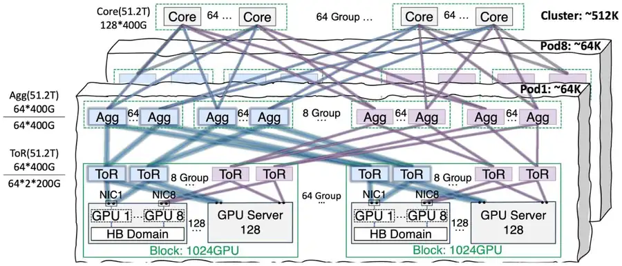
A fifth pattern: Astral. Astral (SIGCOMM 2025) shows that the top tier does not have to be oversubscribed. Its tier 2 joins one rail per group of aggregation switches, which is the option HPN priced at more than 120K GPUs per pod and rejected. A Core tier at 1:1 above it restores the paths between rails. Tencent runs 128K GPUs in two Pods this way, and the design extends to 524,288 GPUs (Figure 13.2; the research notes for this chapter compare it with the four designs).
第五種模式:Astral。Astral(SIGCOMM 2025)說明頂層不一定要超額認購。它的第二層讓每一組聚合交換器只連一條 rail,正是 HPN 算出每個 pod 可超過 120K 顆 GPU、卻否決的那個選項。其上一層 1:1 的 Core 恢復 rail 之間的路徑。騰訊以這種方式在兩個 Pod 中運行 128K 顆 GPU,設計可延伸到 524,288 顆(圖 13.2;本章的研究筆記把它與四種設計比較)。
13.3Axis (b): deep buffers or shallow single chips軸 (b):深緩衝或淺緩衝單晶片
Mechanism. A switch buffer holds packets that arrive faster than the output port can drain them. The time the buffer must cover is the delay of whatever control loop will eventually slow the senders: for DCQCN, one round trip plus up to 50 µs before the first congestion notification packet is sent, plus the slow adaptation of a smoothed estimator with gain 1/256; for PFC, the time until a pause frame reaches the upstream port. A deep-buffer modular chassis has packet memory divided statically among its ports and can hold milliseconds of a 400G burst per port. A single-chip switch has one shared on-chip memory for all its ports: on the order of 100 MB for a 51.2T chip with 128 ports (we round; vendor figures vary), which is about 1 MB per port.
機制。交換器緩衝暫存比輸出埠排空速度更快抵達的封包。緩衝必須涵蓋的時間,是最終會讓發送端減速的那個控制迴圈的延遲:對 DCQCN,是一個往返加上最多 50 µs 才送出第一個壅塞通知封包,再加上增益 1/256 的平滑估計器的緩慢調整;對 PFC,是暫停幀到達上游埠的時間。深緩衝的模組化機箱把封包記憶體靜態分配給各埠,每埠能撐住數毫秒的 400G 突發。單晶片交換器則是所有埠共用一塊晶片內記憶體:128 埠的 51.2T 晶片約在 100 MB 的量級(我們取整;各廠商數字不同),每埠約 1 MB。
Why deep. Meta's spine (CTSW) is a modular chassis with deep buffers. That choice is what let Meta drop DCQCN at 400G when new NIC firmware made it misbehave: the 400G clusters ran for more than a year on PFC alone, and in four years a CTSW never had to send persistent pause frames down to the rack switches. The second half of the mechanism is NCCL's receiver-driven clear-to-send: a sender may post an RDMA write only after the receiver has granted a free channel buffer, so the bytes in flight toward any receiver are bounded in advance. In a 16-to-1 incast test no PFC back-pressure appeared. Note how large Meta's 200G setting already was: a relaxed ECN threshold of 5 MB per port. On a single chip with 128 ports, 5 MB per port would need 640 MB, several times the whole chip's memory. The deep-buffer choice and the no-DCQCN choice are one decision.
為何要深。Meta 的 spine(CTSW)是深緩衝的模組化機箱。這個選擇讓 Meta 在新 NIC 韌體使 DCQCN 行為異常時得以在 400G 放棄它:400G 叢集只靠 PFC 運行超過一年,而四年內 CTSW 從未需要持續向機櫃交換器送出暫停幀。機制的另一半是 NCCL 接收端驅動的 clear-to-send:發送端只有在接收端授予一個空閒 channel 緩衝區後才能提交 RDMA 寫入,所以朝任一接收端的在途位元組事先就有上限。在 16 對 1 的 incast 測試中沒有出現 PFC 反壓。注意 Meta 在 200G 的設定已經有多大:每埠寬鬆的 5 MB ECN 門檻。在 128 埠的單晶片上,每埠 5 MB 需要 640 MB,是整顆晶片記憶體的好幾倍。深緩衝的選擇與不用 DCQCN 的選擇是同一個決策。
Figure 13.3 draws this comparison to scale.
圖 13.3 依比例畫出這個比較。
Why shallow. Alibaba's fleet runs 32.6× more single-chip switches than multi-chip ones, yet the multi-chip switches produced 3.77× more critical hardware failures in total. A single chip is also what makes a 1,024-GPU segment possible in one tier, and single-chip boxes are cheaper. The price is heat and congestion control: the 51.2T chip draws 45% more power than the 25.6T generation at the same 105 °C junction limit, so Alibaba redesigned the vapor chamber for 15% more cooling; and with about 1 MB per port, DCQCN or a successor must stay on. MegaScale, on Tomahawk 4 single chips, kept congestion control and rebuilt it: default DCQCN caused excessive PFC pauses in large all-to-all, so ByteDance combined Swift's precise RTT measurement with DCQCN's fast ECN response.
為何要淺。阿里的機群運行的單晶片交換器數量是多晶片的 32.6 倍,多晶片交換器卻總共產生 3.77 倍的重大硬體故障。單晶片也是讓 1,024 顆 GPU 的 segment 能在一層內成立的原因,而且單晶片盒子更便宜。代價是熱與壅塞控制:51.2T 晶片比 25.6T 世代多耗 45% 功率,接面溫度上限同為 105 °C,所以阿里重新設計均熱板多散 15% 的熱;而每埠約 1 MB 的緩衝下,DCQCN 或其後繼者必須保持開啟。MegaScale 用 Tomahawk 4 單晶片,保留並重建了壅塞控制:預設 DCQCN 在大規模 all-to-all 中造成過多 PFC 暫停,所以字節跳動把 Swift 精確的 RTT 量測與 DCQCN 快速的 ECN 反應結合。
The inequality that decides it. DCQCN only works if the switch marks packets before it has to pause. The DCQCN paper derives the condition: if ingress ports can all feed one egress queue, ECN marking at threshold must happen before any port reaches the PFC threshold, so
決定一切的不等式。DCQCN 只有在交換器必須暫停之前就標記封包時才有效。DCQCN 論文推導出條件:若 個入口埠可能同時餵入同一個出口佇列,在門檻 的 ECN 標記必須先於任何埠達到 PFC 門檻,所以
The PFC threshold itself is bounded by the buffer left after headroom is reserved for every lossless class on every port. On their 32-port, 12 MB switch the bound came out at under 21.75 KB. The lesson generalizes: the ECN threshold is bounded by buffer divided by port count, and a chip that doubles its ports without doubling its memory halves the room for congestion control. Deep buffers make the inequality easy; shallow buffers with 128 ports make it tight.
PFC 門檻本身又受限於為每個埠的每個無損類別保留 headroom 之後剩下的緩衝。在他們 32 埠、12 MB 的交換器上,上界算出 低於 21.75 KB。這個教訓可以推廣:ECN 門檻受緩衝除以埠數的限制,一顆埠數加倍卻記憶體不加倍的晶片,壅塞控制的空間就減半。深緩衝讓不等式輕鬆;128 埠的淺緩衝讓它很緊。
Worked example: an incast at 400G. Sixteen GPUs send to one at 400G each, as in Meta's test, with Meta's measured 22 µs round trip and DCQCN's 50 µs notification interval:
算一題:400G 的 incast。十六顆 GPU 各以 400G 送給同一顆,如 Meta 的測試,並以 Meta 實測的 22 µs 往返與 DCQCN 的 50 µs 通知間隔計:
| Question問題 | Calculation算式 | Result結果 |
|---|---|---|
| Excess arrival rate at the receiver's port, 15 extra senders接收端埠的超量到達率,多出的 15 個發送端 | GB/s | |
| Time before the first rate cut can take effect第一次降速能生效之前的時間 | µs | |
| Bytes that arrive in that time這段時間內到達的位元組 | MB |
54 MB is a large fraction of a shallow chip's entire shared memory and far more than its per-port share, so PFC fires first and the parking-lot and victim-flow problems of PFC return. The same incast on a deep-buffer spine fits in the buffer. With receiver-driven admission, the question does not arise: sixteen senders can have in flight at most sixteen times one connection's channel buffers, which is why Meta observed no PFC in that test.
54 MB 是淺晶片整塊共享記憶體的一大部分、遠超過它的每埠份額,所以 PFC 先觸發,PFC 的停車場與受害者流問題又回來了。同樣的 incast 在深緩衝的 spine 上放得進緩衝。有接收端驅動許可時,這個問題根本不會出現:十六個發送端的在途量最多是一條連線 channel 緩衝區的十六倍,這就是 Meta 在該測試中沒有觀察到 PFC 的原因。
Figure 13.4 plots the queue during these 72 µs. Panel 13.3 lets you change the senders, the port speed and the round trip.
圖 13.4 畫出這 72 µs 內的佇列。面板 13.3 讓你改變發送端數、埠速率與往返時間。
Animation 13.2 plays the same incast on three ports: a shallow chip, a deep-buffer chassis, and a deep chassis with receiver-driven admission.
動畫 13.2 在三種埠上播放同一個 incast:淺晶片、深緩衝機箱,以及加上接收端驅動許可的深緩衝機箱。
13.4Axis (c): fix load balance in software, in wiring, or in circuits軸 (c):以軟體、接線或電路解決負載平衡
Mechanism. A Clos has many equal paths, and a switch picks one per flow by hashing packet headers. With thousands of flows the law of large numbers spreads load evenly. Training produces a few very large flows, about 4 queue pairs per GPU for an AllReduce on 128 GPUs in Meta's measurement, so collisions are common, and in a three-tier network the same header is hashed again at the next tier, which HPN calls hash polarization. There are three ways out. Software: make more flows and hash on more fields. Wiring: build the network so that there is no choice to hash. Circuits: remove packet switching so that there is no shared link at all.
機制。Clos 有許多等價路徑,交換器對封包標頭做雜湊、為每條流挑一條。流有數千條時,大數法則讓負載分得很均勻。訓練產生的是少數非常大的流——Meta 量到 128 顆 GPU 的 AllReduce 每顆 GPU 約 4 個 queue pair——所以碰撞很常見,而三層網路中同一個標頭在下一層會再被雜湊一次,HPN 稱之為 hash polarization。出路有三條。軟體:製造更多的流、對更多欄位做雜湊。接線:把網路建成沒有選擇可雜湊。電路:拿掉封包交換,讓根本沒有共用鏈路。
Figure 13.5 shows how a second hash of the same header leaves links idle.
圖 13.5 畫出對同一個標頭再雜湊一次,如何讓鏈路閒置。
A formula for idle uplinks. If flows are hashed independently onto equal uplinks, the expected number of uplinks that receive no flow is
閒置上行的公式。若 條流各自獨立雜湊到 條等價上行,沒收到任何流的上行數期望值是
For 16 flows on 16 uplinks that is idle uplinks: more than a third of the capacity carries nothing while other uplinks carry two or three flows at half or a third of their rate. With 64 flows the expected idle count falls to 0.26, and with 256 flows to almost zero. This is the arithmetic behind QP scaling: Meta's collective library opens several queue pairs per logical connection, 16 for LLM jobs, and the switch hashes on the destination queue-pair number read from inside the RoCE packet (enhanced ECMP). Idle links disappear, but balance is still probabilistic: Meta's own simulation of 1,000 flows on 16 links left the busiest link at 1.2× the average, and moving from 4 to 32 QPs improved the worst case from 20% to 52% of the optimum while the average stayed about 40% above it.
16 條流在 16 條上行時是 條閒置:超過三分之一的容量什麼都沒載,其他上行卻載著兩三條流、各只剩一半或三分之一速率。64 條流時閒置期望值降到 0.26,256 條時幾乎為零。這就是 QP scaling 背後的算術:Meta 的集體通訊函式庫為每條邏輯連線開多個 queue pair,LLM 任務開 16 個,交換器對從 RoCE 封包內讀出的目的 queue-pair 編號做雜湊(enhanced ECMP)。閒置鏈路消失了,但平衡仍是機率性的:Meta 自己對 16 條鏈路上 1,000 條流的模擬,最忙的鏈路仍是平均的 1.2 倍;從 4 個 QP 增加到 32 個,最差情況從最佳值的 20% 改善到 52%,平均仍比最佳值差約 40%。
Panel 13.4 hashes the flows for you and counts the idle uplinks.
面板 13.4 替你雜湊這些流,並計算閒置的上行。
The software answer, continued. Inside AI Zones Meta added centralized traffic engineering: a controller that knows every flow and assigns each one a path. On 16 uplinks it held utilization near 80% where enhanced ECMP swung between 40% and 90%, and on 128 GPUs it gained 5–10%. Meta did not extend it across the data center: a controller that must react to every failure and job change was judged not worth 5–10%. The paper's closing idea, flowlet switching with a 256–512 µs gap threshold, moves flows during natural gaps with under one reordered packet per second.
軟體答案,續。Meta 在 AI Zone 內加上集中式流量工程:一個知道每條流、為每條流指派路徑的控制器。在 16 條上行上它把使用率穩在 80% 附近,enhanced ECMP 則在 40% 到 90% 之間擺盪;在 128 顆 GPU 上多了 5–10%。Meta 沒有把它擴展到整個資料中心:一個必須對每次故障與任務變動做反應的控制器,被判斷不值 5–10%。論文結尾的想法是 flowlet switching,以 256–512 µs 的空檔門檻在自然空檔時移動流,亂序低於每秒一個封包。
The wiring answer. HPN's dual-plane removes the hash at the aggregation layer by construction: ToR1 of every pair connects only to the 60 aggregation switches of plane 1, ToR2 only to plane 2, so a packet that leaves a plane-1 ToR can only arrive at the destination's plane-1 ToR. Before dual-plane, the two ToR ports toward one NIC carried a 3:1 load ratio with queues of 267 KB against 3 KB; after it they carried equal load, the average queue fell to 20 KB, a 91.8% reduction, and an ablation attributes up to 71.6% of the cross-segment gain to dual-plane. The 60-way choice that remains at the ToR is given to the host, which uses RePaC to find five-tuples with fully disjoint paths and then sends each message on the connection with the smallest count of queued bytes; with four AllReduce jobs on 512 GPUs this gave up to 34.7%. MegaScale took the brute-force wiring answer, 2× uplink bandwidth at the ToR so that collisions no longer saturate a link; this is the same mitigation that Meta used as stage 3 and then abandoned as too expensive.
接線答案。HPN 的 dual-plane 從構造上拿掉聚合層的雜湊:每對的 ToR1 只接平面 1 的 60 台聚合交換器、ToR2 只接平面 2,所以離開平面 1 ToR 的封包只可能到達目的地的平面 1 ToR。在 dual-plane 之前,朝同一張 NIC 的兩個 ToR 埠負載比是 3:1,佇列 267 KB 對 3 KB;之後兩個埠負載相等,平均佇列降到 20 KB、減少 91.8%,消融實驗把跨 segment 增益中最多 71.6% 歸因於 dual-plane。ToR 上剩下的 60 選 1 交給主機,主機用 RePaC 找出路徑完全不相交的五元組,再把每則訊息送到排隊位元組計數最小的連線;四個 AllReduce 任務在 512 顆 GPU 上得到最多 34.7%。MegaScale 採取蠻力的接線答案:ToR 上行頻寬 2 倍,讓碰撞不再塞滿鏈路;這與 Meta 第三階段用過、後來因太貴而放棄的緩解相同。
The circuit answer. TPU v4 has no hash because it has no shared link: a circuit through an OCS belongs to one slice, and routing inside the torus is deterministic dimension-order routing. The price is that a circuit is reserved whether or not it carries data, that reconfiguration takes milliseconds, and that a job's communication pattern must map onto neighbors, which XLA arranges when it picks the collective algorithm for the slice shape. For a training job that keeps the same pattern for days this is a good trade; for mixed traffic it is not.
電路答案。TPU v4 沒有雜湊,因為它沒有共用鏈路:穿過 OCS 的電路屬於一個切片,環面內部的路由是確定性的維度順序路由。代價是電路無論是否承載資料都被保留、重新配置需要毫秒,而且任務的通訊模式必須能映射到鄰居上,這由 XLA 在為切片形狀挑選集體演算法時安排。對一個連續數天維持相同模式的訓練任務這是好交易;對混合流量則不是。
13.5Axis (d): where redundancy lives軸 (d):備援放在哪裡
Mechanism. Every failure of a link, a switch or a host removes bandwidth or a rank from a synchronous job, and the job either slows or stops. Each design places spare capacity somewhere so that the common failures slow the job instead of stopping it, and automates the rest so that the stops are short. The four places are uplink headroom, a second rack switch, a second port on every NIC, and spare compute that a switch can wire in.
機制。每一次鏈路、交換器或主機的故障,都會從同步任務中拿走頻寬或一個 rank,任務要嘛變慢、要嘛停下。每個設計都把備用容量放在某處,讓常見故障只拖慢任務而非停止它,並把其餘的自動化讓停擺很短。四個位置是:上行餘裕、第二台機櫃交換器、每張 NIC 的第二個埠,以及交換器能接進來的備用計算。
Meta: headroom in the uplinks. Meta's rack switch serves one rack, 16 GPUs in Llama 3, and is built at 1:1.125 uplink to downlink bandwidth. Our arithmetic: 16 downlinks of 400G need uplinks of 400G. If two uplinks fail, 16 remain, exactly 1:1, so the job does not slow, which is what the paper states: 1:1.125 tolerates two failed uplinks. The cost is 12.5% more uplink ports and transceivers, against the 100% that the earlier 1:2 design cost. A failed rack switch still stops the rack, and Meta accepts this; the Llama 3 failure table shows that switches and cables caused 8.4% of unexpected interruptions, while GPUs caused 58.7%.
Meta:餘裕放在上行。Meta 的機櫃交換器服務一個機櫃,Llama 3 中是 16 顆 GPU,建成上行對下行 1:1.125。我們的算術:16 條 400G 下行需要 條 400G 上行。若兩條上行故障,剩 16 條、剛好 1:1,任務不會變慢,正如論文所述:1:1.125 容忍兩條上行故障。代價是多 12.5% 的上行埠與光模組,相對於早先 1:2 設計的 100%。機櫃交換器故障仍會停掉整個機櫃,Meta 接受這點;Llama 3 的故障表顯示交換器與線纜造成 8.4% 的非預期中斷,GPU 則造成 58.7%。
HPN: a second switch, and no extra ports. Each HPN NIC has two 200G ports to two rack switches that share no link and no state; the host bonds the ports and sends its address announcements to both. In HPN's test, failing one link removed one of a host's 16 ports and throughput dropped 6.25% and returns the moment the link is repaired, while the single-ToR baseline halted and could not recover if repair took more than two minutes. Dual-ToR costs no extra switch ports: HPN's Table 2 shows 64 GPUs per switch in both the plain Clos and the dual-ToR design, because a pair of switches serves 128 GPUs at half the bandwidth each. What it costs is the host-side bonding and the discipline of never stacking the two switches, since more than 40% of critical failures in Alibaba's older network came from stacked designs. The segment also carries 64 backup GPUs, from the 8 backup 200G ports on each of its 16 ToRs, so a failed host is replaced without leaving the segment.
HPN:第二台交換器,而且不多用埠。每張 HPN NIC 有兩個 200G 埠,接到兩台沒有鏈路也沒有共享狀態的機櫃交換器;主機把兩個埠綁定並向兩台宣告自己。一條鏈路故障拿掉主機 16 個埠中的一個,吞吐下降 6.25%,鏈路修復的瞬間就恢復;單 ToR 基線則停擺,修復超過兩分鐘就無法恢復。Dual-ToR 不多花交換器埠:HPN 的 Table 2 顯示一般 Clos 與 dual-ToR 設計都是每台交換器 64 顆 GPU,因為一對交換器以各一半的頻寬服務 128 顆 GPU。它花的是主機端的綁定,以及永不堆疊兩台交換器的紀律——阿里舊網路超過 40% 的重大故障來自堆疊設計。Segment 還帶著 64 顆備援 GPU,來自 16 台 ToR 各 8 個備援 200G 埠,所以故障主機的替換不必離開 segment。
MegaScale: a standby pool and a loop. ByteDance's redundancy is compute, not network: a standby pool of nodes and a driver that detects, diagnoses, evicts and resumes. The heartbeat carries RDMA traffic counters, so a drop in traffic raises an alert and silence triggers recovery; diagnosis runs NIC loopback and NIC-to-NIC tests, an in-node all-to-all and an all-reduce with the neighbors under the same ToR. In a multi-week run on more than 10,000 GPUs the job restarted more than 100 times, over 90% of faults were handled without a human, and effective training time stayed above 90%.
MegaScale:備用池與一個迴圈。字節跳動的備援是計算而非網路:一個備用節點池,加上一個偵測、診斷、逐出、恢復的 driver。心跳帶著 RDMA 流量計數器,流量下降就警報、完全停止就觸發恢復;診斷執行 NIC 迴路與 NIC 對 NIC 測試、節點內 all-to-all,以及與同一 ToR 下鄰居的 all-reduce。在超過 10,000 顆 GPU 上數週的運行中,任務重啟超過 100 次,超過 90% 的故障不需人介入,有效訓練時間維持在 90% 以上。
TPU v4: spare cubes behind a mirror. A fixed torus has the worst failure behavior of all: one dead host breaks the torus for every job whose slice contains it. Our arithmetic shows how bad. A 1,024-chip slice spans 16 cubes and 256 hosts; a 4,096-chip slice has 1,024 hosts. The probability that every host of a slice is up at a given moment:
TPU v4:鏡片後面的備用 cube。固定環面的故障行為是所有設計中最糟的:一台死掉的主機會讓切片包含它的每個任務的環面斷裂。我們的算術顯示有多糟。一個 1,024 顆晶片的切片橫跨 16 個 cube、256 台主機;4,096 顆晶片的切片有 1,024 台主機。某一時刻切片的每台主機全部可用的機率:
| Question問題 | Calculation算式 | Result結果 |
|---|---|---|
| 1,024-chip slice, 256 hosts, each up 99.5% of the time1,024 顆晶片的切片,256 台主機,每台 99.5% 的時間可用 | ||
| 4,096-chip slice, 1,024 hosts at 99.5%4,096 顆晶片的切片,1,024 台主機,99.5% | ||
| 4,096-chip slice, 1,024 hosts at 99.9%4,096 顆晶片的切片,1,024 台主機,99.9% |
Even at 99.9%, a fixed whole-machine slice is intact only about 36% of the time. This is the mechanism behind the paper's Figure 4, where a fixed torus delivers good goodput only at 99.9% host availability. The OCS changes the question: the scheduler picks any set of working cubes and sets the mirrors, so a slice needs enough working cubes somewhere in the machine, not a specific set of hosts all up at once. Goodput then holds at 99.0–99.5% availability, and a slice of one quarter of the machine still reaches 75%. Eight spare ports per OCS cover switch-side repairs.
即使在 99.9%,固定的整機切片也只有約 36% 的時間完整。這就是論文 Figure 4 背後的機制:固定環面只有在 99.9% 的主機可用性下才有良好的 goodput。OCS 改變了問題:排程器挑任何一組正常的 cube 並設定鏡片,所以切片只需要機器裡某處有足夠的正常 cube,而不是某一組特定主機同時全部可用。於是 goodput 在 99.0–99.5% 的可用性下仍可接受,占整機四分之一的切片仍達 75%。每台 OCS 的 8 個備用埠負責交換器側的維修。
A later Google paper measured this effect on deployed pods (the figure in Section 6.9). Panel 13.5 is a simple model of the same mechanism.
Google 之後的一篇論文在已部署的 pod 上量到這個效應(第 6.9 節的圖)。面板 13.5 是同一機制的簡單模型。
What the numbers say together. The Llama 3 run had 466 interruptions in 54 days and still kept effective training time above 90%. Our arithmetic:
這些數字合起來說什麼。Llama 3 的運行在 54 天內有 466 次中斷,有效訓練時間仍高於 90%。我們的算術:
| Question問題 | Calculation算式 | Result結果 |
|---|---|---|
| Average spacing of 466 interruptions in 54 days54 天 466 次中斷的平均間隔 | h小時 | |
| Most lost time that 90% effective time allows90% 有效時間所允許的最多損失時間 | min分鐘 | |
| Average cost per interruption每次中斷的平均代價 | min分鐘 |
So the average interruption, one every 2.8 hours, including detection, replacement and the restart from the last checkpoint, cost less than 17 minutes. Only 3 of 466 needed a person. MegaScale reports the same shape: under 10 minutes to diagnose and 15 minutes to catch up. Redundancy in the network buys the first few percent; automation of the restart buys the rest.
所以平均每 2.8 小時一次的中斷——包含偵測、替換與從最後檢查點重啟——每次代價低於 17 分鐘。466 次中只有 3 次需要人。MegaScale 報告同樣的形狀:診斷低於 10 分鐘、追回 15 分鐘。網路中的備援買到前幾個百分點;重啟的自動化買到其餘。
Animation 13.3 plays one failure sequence in each design and shows where the traffic or the work goes.
動畫 13.3 為每種設計播放一段故障過程,並顯示流量或工作移到哪裡。
HPN's dual-ToR and Meta's 1:1.125 headroom both protect against link failures. Which one also protects against a rack-switch failure, which one costs extra switch ports, and which one protects against a failed GPU? Use the matrix rows "ToR redundancy" and "Failure handling", then check your answer against the risk line that Panel 13.7 prints for each pattern.
HPN 的 dual-ToR 與 Meta 的 1:1.125 餘裕都防鏈路故障。哪一個也防機櫃交換器故障?哪一個要多花交換器埠?哪一個防 GPU 故障?用矩陣的「ToR 備援」與「故障處理」兩列作答,再對照面板 13.7 為每種模式印出的風險那一行。
13.6Where the designs agree設計之間一致的地方
The disagreements above are loud, but the agreements are what a designer should copy first, because four independent teams reached them from different starting points.
上面的分歧很響亮,但一致之處才是設計者該先抄的,因為四個獨立團隊從不同起點得到了相同的結論。
- Optics are a small share of the bill. Google's whole optical fabric, OCSes included, is under 5% of system cost and under 3% of power. The rail-only paper's coefficients make a transceiver ($199) less than a third of a switch port ($694). HPN keeps every fiber under 100 m so that multi-mode transceivers, 70% cheaper than single-mode, can be used. The accelerators dominate the cost; the network's job is to keep them busy.光學只占帳單一小部分。Google 的整個光學網路(含 OCS)不到系統成本的 5%、功耗的 3%。Rail-only 論文的係數讓一個光模組(199 美元)不到交換器埠(694 美元)的三分之一。HPN 讓每條光纖都在 100 m 以內,以便使用比單模便宜 70% 的多模光模組。加速器主宰成本;網路的工作是讓它們忙碌。
- Keep heavy traffic local by placement. Meta's scheduler assigns ranks to minimize the traffic across the cut between zones. Llama 3 orders parallelism [TP, CP, PP, DP] so that only prefetchable FSDP traffic crosses the 1:7 links. HPN lets only pipeline traffic, 6 MB per step against 5.5 GB for data parallelism, cross pods at 15:1. MegaScale places communication-heavy ranks under one ToR set. TPU v4 gives a pipeline job a 4×4×32 "cigar" slice. The topology sets the ceiling; placement decides how close the job gets to it.靠配置讓重流量留在本地。Meta 的排程器指派 rank 讓跨 zone 切割的流量最少。Llama 3 以 [TP, CP, PP, DP] 排列平行化,只讓可預先抓取的 FSDP 流量跨越 1:7 鏈路。HPN 只讓管線流量——每步 6 MB,對比資料平行的 5.5 GB——以 15:1 跨 pod。MegaScale 把通訊密集的 rank 放在同一組 ToR 下。TPU v4 給管線任務一個 4×4×32 的「雪茄」切片。拓樸決定天花板;配置決定任務離天花板多近。
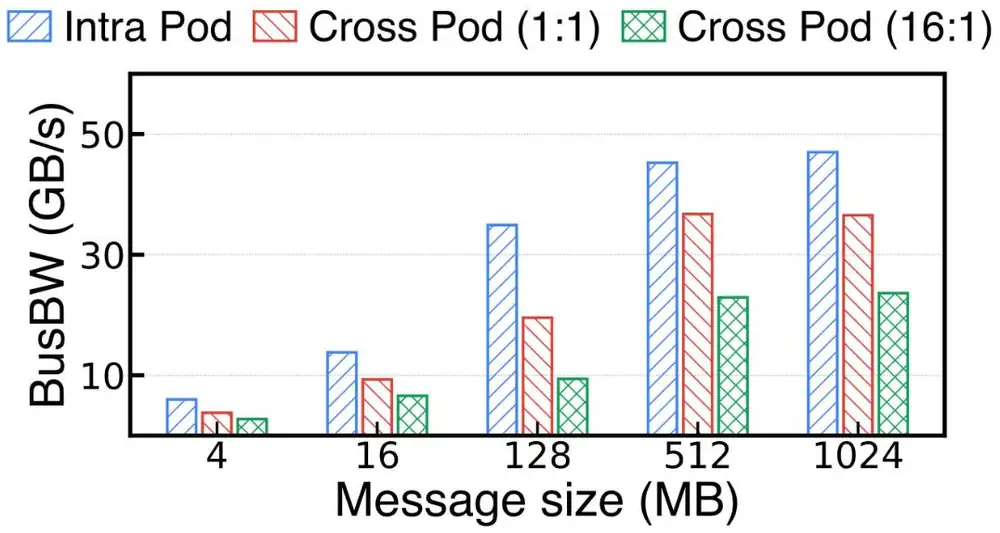
Astral (SIGCOMM 2025) measured both halves of this rule on 1K GPUs (Figure 13.6). Spreading a job over 32 Pods cut all-to-all bandwidth by 19%–37% even with a 1:1 Core, and a 16:1 Core cut up to 52% more. So Tencent keeps its top tier at 1:1: an oversubscribed top tier is the cheap choice, not a forced one.
Astral(SIGCOMM 2025)在 1K 顆 GPU 上量到這條規則的兩半(圖 13.6)。把任務分散到 32 個 Pod,即使 Core 為 1:1,all-to-all 頻寬也少 19%–37%;Core 為 16:1 時再少最多 52%。所以騰訊把頂層維持在 1:1:超額認購的頂層是便宜的選擇,不是被迫的選擇。
Panel 13.6 shows why HPN lets only pipeline traffic cross its 15:1 core.
面板 13.6 說明 HPN 為什麼只讓管線流量跨越 15:1 的核心層。
- Bound the bytes in flight. Meta's receiver-driven clear-to-send caps unacknowledged data at a fixed number of channel buffers per connection. IRN's BDP-FC caps each queue pair at one bandwidth-delay product (120 KB at 40G; about 1.1 MB at 400G with a 22 µs RTT). HPN's host keeps a counter of queued bytes per connection and sends on the smallest. TPU links are credit-based. All four prevent queues instead of reacting to them.限制在途位元組。Meta 接收端驅動的 clear-to-send 把未確認資料限制在每條連線固定數量的 channel 緩衝區。IRN 的 BDP-FC 把每個 queue pair 限制在一個頻寬延遲乘積(40G 時 120 KB;400G 與 22 µs RTT 時約 1.1 MB)。HPN 的主機為每條連線維護排隊位元組計數器並從最小者發送。TPU 鏈路以 credit 為基礎。四者都是預防佇列而非事後反應。
- Separate the front end from the back end. Meta's Tectonic, HPN's ninth NIC, MegaScale's HDFS and TPU's CPU hosts all keep storage, checkpoints and management off the training fabric. HPN tried the opposite and saw training fluctuate. The front end must still absorb a checkpoint burst: Tectonic's 7 TB/s peak exists for the moment when 16,000 GPUs write at once.把前端與後端分開。Meta 的 Tectonic、HPN 的第九張 NIC、MegaScale 的 HDFS 與 TPU 的 CPU 主機,都把儲存、檢查點與管理留在訓練網路之外。HPN 試過相反的做法,看到訓練波動。前端仍必須吸收檢查點突發:Tectonic 的 7 TB/s 峰值就是為 16,000 顆 GPU 同時寫入的那一刻而存在。
- Automate recovery. 3 of 466 interruptions needed a human at Meta; over 90% were automatic at ByteDance; HPN turned a switch failure into a 6.25% slowdown; Google's scheduler rewires around a dead cube. None of the four tried to make failures rare; all four made them cheap.把恢復自動化。Meta 的 466 次中斷只有 3 次需要人;字節跳動超過 90% 自動處理;HPN 把交換器故障變成 6.25% 的減速;Google 的排程器繞過死掉的 cube 重新接線。四者都沒有試圖讓故障罕見;四者都讓故障變便宜。
- Measure everything. Meta watches out-of-sequence counters, link flaps, ACK timeouts, a PFC watchdog at 200 ms and buffer alarms at 80%. HPN sends INT probes that record switch and port at every hop and compares them with the wiring blueprint. MegaScale puts RDMA counters in every heartbeat and times every rank with CUDA events, which found the 0.5% of machines that were 10% slow. Llama 3 keeps an NCCL flight recorder. The slowest link or rank sets the pace of thousands of GPUs, so the instrument that finds it pays for itself.量測一切。Meta 監看亂序計數器、鏈路抖動、ACK 逾時、200 ms 的 PFC watchdog 與 80% 的緩衝警報。HPN 送出在每一跳記錄交換器與埠的 INT 探測封包,並與接線藍圖比對。MegaScale 在每次心跳放入 RDMA 計數器,並用 CUDA 事件為每個 rank 計時,找出了慢 10% 的那 0.5% 機器。Llama 3 保留 NCCL flight recorder。最慢的鏈路或 rank 決定數千顆 GPU 的節奏,所以找出它的儀器自己就划得來。
13.7A decision procedure一套決策程序
The inputs are things you know before you buy anything: the target GPU count now and in three years; the building's power limit; the model types you will train, including the share that are mixture-of-experts; whether hosts are shared between tenants; whether your team can operate a traffic-engineering controller or custom NIC firmware and whether it can maintain a fork of the collective library; how sensitive the project is to network cost; and which switch-chip generation you can buy. The outputs are the rows of the matrix: tiers, switch class, ToR redundancy, load-balancing scheme and congestion-control scheme. Work through the steps in order. Each threshold is a number from one of the papers.
輸入是你在買任何東西之前就知道的事:現在與三年後的目標 GPU 數;建築的電力上限;要訓練的模型類型,包括混合專家模型的占比;主機是否在租戶之間共享;團隊能否運行流量工程控制器或自製 NIC 韌體、能否維護集體通訊函式庫的分支;專案對網路成本有多敏感;以及你買得到哪一代交換晶片。輸出就是矩陣的列:層數、交換器類別、ToR 備援、負載平衡方案與壅塞控制方案。依序走完這些步驟。每個門檻都是某篇論文裡的數字。
- Count GPUs against the scale units. Up to 1,024: one 51.2T segment gives every same-rail transfer one switch hop and no second-tier hashing; 96.3% of Alibaba's jobs fit here. Up to 3,072: one Meta-style zone or pod with full bisection. Up to 4,096: one torus machine, if you own the whole stack. Up to 15,000: one HPN pod, two tiers, dual-plane. From 15K to about 24K: the 2024 designs oversubscribe the top tier, 1:7 (Meta) and 15:1 (HPN), and both worked because placement kept all but PP or DP traffic below it. This is the cheap choice, not the only one: Astral runs 128K GPUs under a 1:1 Core (Section 13.2). Above 32K: this is where rail-only's savings are largest and where the 2024 designs end; HPN's stated target is 100K and Meta's 24K design was replaced for 100K+.把 GPU 數對照規模單位。1,024 以內:一個 51.2T segment 讓每次同 rail 傳輸只跨一台交換器、沒有第二層雜湊;阿里 96.3% 的任務落在這裡。3,072 以內:一個具完整對分的 Meta 式 zone 或 pod。4,096 以內:一台環面機器,前提是你擁有整個堆疊。15,000 以內:一個 HPN pod,兩層、dual-plane。15K 到約 24K:2024 年的設計都讓頂層超額認購,1:7(Meta)與 15:1(HPN),兩者都行得通,因為配置讓除了 PP 或 DP 之外的流量都留在它之下。這是便宜的選擇,不是唯一的選擇:Astral 在 1:1 的 Core 之下運行 128K 顆 GPU(第 13.2 節)。32K 以上:這是 rail-only 節省最大的地方,也是 2024 年設計的終點;HPN 宣稱的目標是 100K,Meta 的 24K 設計則已為 100K+ 而被取代。
- Check the building. HPN's rule of thumb is 18 MW per building for about 15,000 GPUs, which is 1.2 kW per GPU all-in. Divide your power limit by 1.2 kW to get the GPUs one building can hold; if the target exceeds it, the top tier must cross buildings, and fibers over 100 m lose the 70% multi-mode saving. HPN sized its pod to the building on purpose.檢查建築。HPN 的經驗法則是每棟建築 18 MW、約 15,000 顆 GPU,即全包每顆 GPU 1.2 kW。把你的電力上限除以 1.2 kW 得到一棟建築能容納的 GPU 數;若目標超過,頂層就必須跨建築,超過 100 m 的光纖也會失去 70% 的多模節省。HPN 刻意把 pod 的大小訂成一棟建築。
Figure 13.7 puts steps 1 and 2 on one axis.
圖 13.7 把第 1 與第 2 步放在同一條軸上。
- Check the workload mix and the tenancy. If any meaningful share of the work is mixture-of-experts, or if hosts are shared, keep an any-to-any tier above the rails: rail-only slows MoE all-to-all by 8.2–11.2% and cannot relay across tenants, and a torus needs twisting to serve all-to-all at all. Rail-only is a choice only for single-tenant clusters with a placement discipline you can enforce. For MoE that discipline exists in production: DeepSeek-V3 sends each token to at most 4 nodes and forwards it over NVLink, on eight planes that never meet, and trained as fast as on a network whose rails meet; MegaScale-MoE keeps expert parallelism inside the node (Chapter 3, Section 13.7).檢查工作負載組成與租戶模式。若有任何可觀比例的工作是混合專家模型,或主機被共享,就在 rail 之上保留一個任意對任意的層:rail-only 讓 MoE 的 all-to-all 慢 8.2–11.2%、也無法跨租戶中繼,而環面要服務 all-to-all 根本需要扭轉。Rail-only 只在單租戶、且你能強制配置紀律的叢集才是選項。對 MoE,生產環境已有這種紀律:DeepSeek-V3 讓每個 token 最多送到 4 個節點、再經 NVLink 轉送,跑在互不相連的八個平面上,訓練速度與 rail 彼此相連的網路相同;MegaScale-MoE 則把專家平行留在節點內(第 3 章、第 13.7 節)。
- Pick the switch class, and the congestion control follows. Deep-buffer modular spines let you run 400G with PFC plus receiver-driven admission and without DCQCN, as Meta did for more than a year; they cost more and, in Alibaba's fleet, failed 3.77× more often. Shallow single chips give one tier of 1,024 GPUs and fewer failures, but you keep DCQCN or a hybrid such as MegaScale's Swift-plus-DCQCN, and you must respect : the ECN threshold cannot exceed the buffer divided by the port count, so set it low, keep PFC watchdogs at about 200 ms, and never put broadcast traffic in a lossless class.選交換器類別,壅塞控制隨之決定。深緩衝的模組化 spine 讓你像 Meta 那樣以 PFC 加接收端驅動許可、不用 DCQCN 跑 400G 超過一年;它們更貴,而且在阿里的機群中故障多 3.77 倍。淺的單晶片給你一層 1,024 顆 GPU 與更少的故障,但你得保留 DCQCN 或像 MegaScale 的 Swift 加 DCQCN 這類混合,並且必須遵守 :ECN 門檻不能超過緩衝除以埠數,所以把它設低、PFC watchdog 維持約 200 ms,永不把廣播流量放進無損類別。
- Choose how to beat the hash. If you can change both the switch hash and the collective library, use QP scaling with 16 flows per pair and hash on the destination QP (up to 40%). If you can dictate the wiring, use dual-plane and host-side path selection (91.8% shorter queues, +34.7% under contention). If you have a controller team, add traffic engineering inside the non-blocking domain (+5–10%) and no further. If you can do none of these, buy 2× uplinks and accept the cost, as MegaScale did.決定怎麼打敗雜湊。若你能同時改交換器雜湊與集體通訊函式庫,用每對 16 條流的 QP scaling 並對目的 QP 雜湊(最多 40%)。若你能決定接線,用 dual-plane 加主機端選路(佇列短 91.8%,競爭下 +34.7%)。若你有控制器團隊,在非阻塞 domain 內加流量工程(+5–10%),到此為止。若以上都做不到,買 2 倍上行並接受成本,如 MegaScale。
Figure 13.8 draws steps 3 to 5 as a tree.
圖 13.8 把第 3 到第 5 步畫成一棵樹。
- Place the redundancy. Pick one of: 1:1.125 uplink headroom (survives two uplink failures, 12.5% more uplinks), non-stacked dual-ToR (survives a rack switch at 6.25%, no extra switch ports, host-side bonding required), or spare compute behind a reconfigurable switch (OCS). In every case automate the restart loop and measure effective training time; the production runs held it above 90% with a failure every few hours.放置備援。三選一:1:1.125 的上行餘裕(撐過兩條上行故障,多 12.5% 上行)、非堆疊 dual-ToR(以 6.25% 撐過機櫃交換器故障,不多花交換器埠,需主機端綁定),或可重構交換器(OCS)後面的備用計算。無論哪一種,都把重啟迴圈自動化並量測有效訓練時間;生產運行在每幾小時一次故障下仍維持在 90% 以上。
- Size the front end for the checkpoint burst. Keep it separate. Estimate the burst as GPUs × checkpoint bytes per GPU (1 MB to 4 GB in Llama 3) over the pause you can afford, or stage through host memory as MegaScale does so that the GPUs pause for seconds and HDFS drains in the background.依檢查點突發調整前端大小。保持獨立。把突發估成 GPU 數 × 每顆 GPU 的檢查點位元組(Llama 3 中 1 MB 到 4 GB)除以你能承受的暫停時間,或像 MegaScale 一樣先經主機記憶體分段,讓 GPU 只暫停數秒、HDFS 在背景排空。
- Account for the chip generation. A 102.4T chip doubles the GPUs per switch and therefore the segment; 800G per GPU halves them back. Run Panel 13.1 with your generation before fixing the pod size, and check the result against step 2.把晶片世代算進去。102.4T 晶片讓每台交換器的 GPU 數加倍、segment 因此加倍;每顆 GPU 800G 又把它減半。在定下 pod 大小之前,用你的世代跑一次面板 13.1,再對照第 2 步檢查結果。
Panel 13.7 encodes these steps as explicit rules and scores the four patterns. The rules are deliberately simple and visible; the point is to see which constraint moves the ranking, not to trust the score.
面板 13.7 把這些步驟編成明確的規則,為四種模式評分。規則刻意簡單且可見;重點是看哪個限制條件會移動排名,而不是信任分數。
In Panel 13.7, start from the defaults and change one input at a time. Which single change moves rail-only from last to first? Which single change moves Meta-style from last to first? Then set the MoE share to 50% and see whether any setting of the other inputs still makes rail-only win. Section 13.2 explains why it should not.
在面板 13.7 從預設值出發,一次只改一個輸入。哪一個改動能把 rail-only 從最後推到第一?哪一個改動能把 Meta 式從最後推到第一?接著把 MoE 占比設成 50%,看看其他輸入的任何設定是否仍能讓 rail-only 勝出。第 13.2 節解釋了為什麼不應該。
13.8What changed after these papers這些論文之後改變了什麼
The four designs are from 2023 and 2024, and several of their fixed points have moved since. Treat this section as direction, not as data. HPN's authors wrote that the next generation is planned around 102.4 Tb/s chips, which, by the arithmetic of Panel 13.1, doubles the GPUs a single tier can hold at 400G; NICs at 800G per GPU halve that gain and push the same question up one tier. Panel 13.8 shows the same effect on the number of tiers.
這四種設計來自 2023 與 2024 年,其中幾個固定點之後已經移動。把這一節當成方向,而不是數據。HPN 的作者寫到下一代圍繞 102.4 Tb/s 晶片規劃,依面板 13.1 的算術,在 400G 下這讓單一層能容納的 GPU 數加倍;每顆 GPU 800G 的 NIC 把這個增益減半,並把同樣的問題往上推一層。面板 13.8 顯示同一個效應在層數上的樣子。
The Ultra Ethernet transport (specification 1.0, 2025) standardizes what IRN argued for in 2018: selective retransmission, a bounded window, and packet spraying across paths, which attacks the low-entropy problem at its root instead of adding hash inputs (Figure 13.9); Chapter 7 covers it. Pegasus (SIGCOMM 2026) is one production form of this idea: per-packet spraying and receiver credits inside Tencent's own NIC (Pegasus, SIGCOMM 2026).
Ultra Ethernet 傳輸層(規範 1.0,2025 年)把 IRN 在 2018 年主張的東西標準化:選擇性重傳、有上限的視窗,以及跨路徑的封包噴灑——從根本上對付低熵問題,而非增加雜湊輸入(圖 13.9);第 7 章有介紹。Pegasus(SIGCOMM 2026)是這個想法的一種生產形式:在騰訊自研的 NIC 內做逐封包噴灑與接收端 credit(Pegasus,SIGCOMM 2026)。
Meta described at SIGCOMM 2026 the communication stack it built for clusters beyond 100,000 GPUs; the research notes on collectives summarize it, and this chapter quotes no numbers from it. Optical circuit switching, which TPU v4 used inside one machine, entered Google's general data-center fabric in Jupiter (SIGCOMM 2022), and TPU v5p and later generations keep the torus-plus-OCS design. None of this changes the axes in Section 13.2 to 5; it moves where on each axis the cheap option sits.
Meta 在 SIGCOMM 2026 描述了面向十萬顆以上 GPU 叢集的網路與傳輸層,取代本章比較的 enhanced ECMP 加不用 DCQCN 的設計;我們不引用其中任何數字。TPU v4 在單一機器內使用的光路交換,已進入 Google 的通用資料中心網路 Jupiter(SIGCOMM 2022),TPU v5p 與之後的世代也維持環面加 OCS 的設計。這些都沒有改變第 2 到第 13.5 節的軸;它們改變的是每條軸上便宜的選項落在哪裡。
Four production designs answer the same questions differently, and each answer is forced by a constraint the team could not change. Reachability: Meta and HPN keep an any-to-any tier because mixture-of-experts traffic and shared hosts need it; rail-only deletes the spine for dense models; TPU v4 uses a torus with optical switches. Buffers: Meta's deep-buffer spine plus NCCL's clear-to-send let it drop DCQCN; HPN chose reliable single chips and removed overload by wiring. Load balance: more entropy (Meta), fewer choices (HPN), or dedicated circuits (TPU v4). Redundancy: spare uplinks, a second ToR, a standby pool, or spare cubes. All agree on the essentials: keep traffic local, thin only the links that small or tolerant traffic crosses, bound the bytes in flight, separate the front end, and automate recovery.
四個生產設計以不同方式回答同一組問題,每個答案都是由團隊無法改變的限制所決定。可達性:Meta 與 HPN 保留任意對任意的一層,因為混合專家的流量與共用主機需要它;rail-only 為稠密模型拿掉 spine;TPU v4 用搭配光路交換器的環面。緩衝:Meta 的深緩衝 spine 加上 NCCL 的 clear-to-send 讓它能拿掉 DCQCN;HPN 選擇可靠的單晶片,並以接線消除超載。負載平衡:更多熵(Meta)、更少選擇(HPN),或專用電路(TPU v4)。備援:多餘的上行、第二台 ToR、待命池,或備用 cube。所有設計都同意幾件要事:讓流量留在本地、只讓小量或耐延遲流量跨越的鏈路變細、限制在途位元組、把前端分開,以及讓恢復自動化。
The research notes go beyond the four designs: each one picks up a chapter and follows the papers published since. The guided readings retell each production paper in full.
研究筆記超越這四個設計:每一篇接續某一章,追蹤之後發表的論文。導讀則完整重述每一篇生產論文。