Models and simulation: predicting step time before the hardware exists模型與模擬:在硬體存在之前預測步驟時間
Learn the kinds of evidence behind the numbers in this book, build the two-line model of a training step, see what a simulator adds, and check a model against measurements.了解本書數字背後的證據種類,建立訓練步驟的兩行模型,看看模擬器多提供了什麼,並用量測檢驗模型。
This chapter builds on Chapters 4, 5, 6, 11. These earlier terms appear most often below; each chip links to its definition.
New terms in this chapter (3)本章新名詞(3)
Each term is defined in the text where it first appears; the link jumps there. Terms from earlier chapters are listed under "Before you start".
每個名詞都在它第一次出現的段落中定義,點連結可跳過去。前面各章的名詞列在「開始之前」。
- Analytical model解析模型 A formula that predicts a quantity, such as step time, from a few parameters. 以少數參數預測某個量(例如步驟時間)的公式。
- Simulation, packet-level simulation模擬、封包層級模擬 Running a model of the workload and network in software; a packet-level simulator follows every packet through every queue. 以軟體執行工作負載與網路的模型;封包層級模擬器追蹤每個封包經過每個佇列。
- Validation驗證 Checking a model or simulator against measurements of the real system. 以真實系統的量測檢驗模型或模擬器。
12.1Four kinds of evidence四種證據
A measured number comes from real hardware, and it is only as general as the setup it came from: 256 GPUs in a test say little about 16,384 in production. A computed number comes from an analytical model: a formula, such as the α–β model of Chapter 4 or the 6ND rule of Chapter 1, that turns a few parameters into a prediction. It is fast and transparent, and it is only as good as its assumptions. A simulated number comes from a simulator: a program that imitates the hardware piece by piece, packet by packet or collective by collective. It captures interactions that a formula leaves out, at the cost of speed and of many inputs that must be right. Validation is the step that connects them: running a model or simulator on a case that was also measured and comparing the two. A model that has not been validated is a hypothesis. When a paper reports a gain, ask which kind of number it is, and for a computed or simulated one, against what measurement it was validated.
量測的數字來自真實硬體,而它的通用性只和它的實驗設定一樣:測試中的 256 顆 GPU,對生產環境的 16,384 顆說明不了多少。計算的數字來自分析模型:一條公式,例如第 4 章的 α–β 模型或第 1 章的 6ND 法則,把少數幾個參數變成預測。它快速又透明,但只和它的假設一樣可靠。模擬的數字來自模擬器:一個逐一模仿硬體的程式,一次一個封包或一次一個集體操作。它能捕捉公式遺漏的交互作用,代價是速度,以及許多必須正確的輸入。驗證把兩者連起來:在一個同樣有量測結果的案例上執行模型或模擬器,並比較兩者。沒有經過驗證的模型只是假說。當論文報告一個增益時,先問它是哪一種數字;若是計算或模擬所得,再問它是對照哪一個量測驗證過的。
12.2The two-line model兩行模型
Nobody experiments on the real cluster: it costs billions, a production run occupies it for weeks (HPN's 14.9% measurement meant moving a live 2,300-GPU job between networks), and a failed experiment wastes every tenant's GPU-hours, not only the experiment's. So designers estimate first, at two levels: an analytic model you can do on paper, and a simulator that replays the job on a modeled network.
沒有人在真實叢集上做實驗:它價值數十億,一次生產運行占用它數週(HPN 14.9% 的量測意味著把一個活著的 2,300 顆 GPU 任務在網路之間搬動),而失敗的實驗浪費每一個租戶的 GPU 時數,不只是實驗本身的。所以設計者先估計,分兩個層次:可以在紙上做的解析模型,以及在建模網路上重播任務的模擬器。
Start with the – model of one collective:
從單一集體操作的 – 模型開始:
where is the per-round latency, rounds is the number of sequential message exchanges, and is the bandwidth one GPU actually gets. For a ring all-reduce over GPUs with bytes each, and . is the raw link rate divided by a slowdown factor that captures hash collisions, pauses and sharing with other jobs. Then combine communication with computation: part of it hides behind compute and the rest is exposed:
其中 是每回合延遲,回合數是依序的訊息交換次數, 是一顆 GPU 實際得到的頻寬。對 顆 GPU、各 位元組的環狀 all-reduce,,。 是原始鏈路速率除以減速因子 , 涵蓋雜湊碰撞、暫停與和其他任務的共用。然後把通訊與計算結合:一部分藏在計算後面,其餘是暴露的:
MFU relative to compute-only is ; absolute MFU multiplies by the efficiency of the kernels themselves.
相對於純計算的 MFU 是 ;絕對 MFU 再乘上 kernel 本身的效率。
Put HPN's numbers in: , , (Meta's measured fabric round trip), for a 400G NIC, ; compute takes 1 s and 80% of communication is hidden. Then set , as a bad hash collision would. One term per row:
放進 HPN 的數字:、、(Meta 實測的網路往返)、400G NIC 的 、;計算需要 1 s、80% 的通訊被隱藏。然後把 設為 2,像一次糟糕的雜湊碰撞那樣。每列一項:
| Question問題 | Calculation算式 | Result結果 |
|---|---|---|
| DP latency termDP 延遲項 | ms | |
| DP bandwidth termDP 頻寬項 | ms | |
| DP all-reduce DP 的 all-reduce | ms | |
| TP: 560 MB over NVLink at about 450 GB/sTP:560 MB 走約 450 GB/s 的 NVLink | ms | |
| PP: 6 MB over the NICPP:6 MB 走 NIC | ms | |
| Communication per step每步通訊合計 | ms99% of it the DP all-reduce其中 99% 是 DP 的 all-reduce | |
| Exposed communication, 80% hidden暴露的通訊,80% 被隱藏 | ms | |
| Step with 1 s of compute計算 1 s 時的步時間 | srelative MFU ≈ 95.3%相對 MFU ≈ 95.3% | |
| DP bandwidth term at 時的 DP 頻寬項 | ms | |
| Exposed communication at 時暴露的通訊 | ms | |
| Step at 時的步時間 | srelative MFU ≈ 91.5%相對 MFU ≈ 91.5% |
Communication totals about 243 ms per step, 99% of it the DP all-reduce, and with 80% hidden the step is 1.049 s: relative MFU is 95.3%. A factor of two on the network doubles the DP bandwidth term to 440 ms, exposed time grows from 49 to 93 ms, and relative MFU falls to 91.5%. Nearly four MFU points from one factor of two on the network is the size of effect the papers measure, and why the slowdown factor is the right thing to simulate. Figure 12.1 draws the model.
通訊每步合計約 243 ms,其中 99% 是 DP 的 all-reduce;隱藏 80% 之後步時間是 1.049 s,相對 MFU 是 95.3%。網路上的二倍因子讓 DP 頻寬項加倍到 440 ms,暴露時間從 49 ms 增到 93 ms,相對 MFU 降到 91.5%。網路上一個二倍的因子換來將近四個 MFU 百分點:這就是論文量到的效應大小,也是為什麼減速因子是該模擬的對象。圖 12.1 畫出這個模型。
12.3What a simulator adds模擬器多提供了什麼
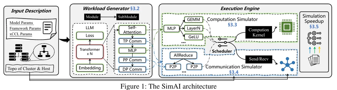
The two-line model treats the network as one number, . A simulator computes from the mechanisms. It needs three inputs: the model and its parallel layout, which give the sequence of compute kernels and communication calls; the collective algorithm, which turns each call into flows between specific ranks; and the network, which carries the flows. A flow-level simulator shares each link's bandwidth among the flows on it and is fast enough for 10,000 GPUs. A packet-level simulator, usually built on ns-3, models queues, ECMP hashing, PFC pauses and DCQCN marking packet by packet; it is far slower but it is the only level that reproduces hash polarization or a victim flow. Alibaba's SimAI (NSDI 2025, Figure 8) runs the real training framework and NCCL on one host to record the exact sequence of operations, then replays it in a packet-level network simulator. ASTRA-sim is the open-source academic tool with pluggable network back ends. Both still depend on a compute model, usually profiled kernel times, and on the fidelity of the collective model, so treat simulated MFU as a comparison between designs rather than a prediction.
兩行模型把網路當成一個數字 。模擬器從機制算出 。它需要三種輸入:模型與其平行配置,給出計算 kernel 與通訊呼叫的序列;集體通訊演算法,把每次呼叫變成特定 rank 之間的流;以及承載這些流的網路。流級模擬器把每條鏈路的頻寬分給其上的流,快到足以處理 10,000 顆 GPU。封包級模擬器通常建在 ns-3 上,逐封包模擬佇列、ECMP 雜湊、PFC 暫停與 DCQCN 標記;它慢得多,但它是唯一能重現 hash polarization 或受害者流的層級。阿里的 SimAI(NSDI 2025,圖 12.2)在單一主機上執行真實的訓練框架與 NCCL 以記錄精確的操作序列,再在封包級網路模擬器裡重播。ASTRA-sim 是可插換網路後端的開源學術工具。兩者仍依賴計算模型(通常是剖析得到的 kernel 時間)與集體模型的精確度,所以把模擬出的 MFU 當作設計之間的比較,而不是預測。
12.4Validating against measurements以量測驗證
A model is worth what it predicts, so check it against the measured numbers. MegaScale's Table 3 is an ablation on 256 GPUs: from a 47.7% baseline, overlapping tensor-parallel communication added 2.2 MFU points, pipeline overlap 2.5 and data-parallel overlap 1.5, a total of 6.2 points from hiding communication; the rest of the climb to 65.3% came from model and operator changes. In the two-line model those 6.2 points are the move from a low overlap fraction to a high one with everything else fixed. MegaScale's Table 2 is the scaling curve: 65.3% at 256 GPUs falls to 55.2% at 12,288. The ring model's latency term alone does not produce a 10-point decline; to reproduce it you must raise with scale, which is a way of saying that collisions, pauses and stragglers grow with the job. Meta's co-tuning result is the most direct test of the term: NCCL's defaults assumed a round trip under 10 µs, the fabric delivered about 22 µs, and the default channel buffers could not keep a 400G link busy; fixing the buffers and prioritizing the clear-to-send message gave more than 2× in many cases.
模型的價值在於它預測什麼,所以拿量到的數字檢驗它。MegaScale 的 Table 3 是 256 顆 GPU 上的消融:從 47.7% 的基線開始,重疊張量平行通訊加 2.2 個 MFU 百分點、管線重疊 2.5、資料平行重疊 1.5,隱藏通訊合計 6.2 點;其餘爬到 65.3% 的部分來自模型與運算子的改動。在兩行模型中,那 6.2 點就是其他條件不變、重疊率從低到高的移動。MegaScale 的 Table 2 是擴展曲線:256 顆 GPU 的 65.3% 降到 12,288 顆的 55.2%。環模型的延遲項本身不會產生 10 點的下降;要重現它必須讓 隨規模上升,這等於是說碰撞、暫停與 straggler 隨任務一起成長。Meta 的共同調校結果是對 項最直接的測試:NCCL 的預設假設往返低於 10 µs,網路給的是約 22 µs,預設的 channel 緩衝塞不滿 400G 鏈路;修正緩衝並讓 clear-to-send 訊息優先,在許多情況下帶來超過 2 倍。
The last check is the gap between a collective benchmark and a training step. HPN's AllReduce on 448 GPUs improved by up to 59.3% when a segment held the whole job, but the production job improved 14.9%. Both numbers are right: the step contains compute that did not change, and most of the collective was already hidden. The relation is so a 59.3% collective gain on a step with roughly a quarter of its time exposed gives about 15%. The panel below is the two-line model with the measured points drawn on top.
最後一項檢驗是集體通訊基準與訓練步之間的差距。HPN 在 448 顆 GPU 上的 AllReduce 在整個任務放進一個 segment 時最多改善 59.3%,但生產任務改善 14.9%。兩個數字都對:步裡包含沒有改變的計算,而大部分集體操作本來就被隱藏。關係是 所以在一個約四分之一時間暴露的步上,59.3% 的集體操作增益大約給 15%。下面的面板就是兩行模型,上面疊著量到的點。
Leave the defaults, which put the curve through MegaScale's 256-GPU point, and move the GPU slider to 8,192 and then 16,384. How far must the slowdown factor rise before the curve meets MegaScale's 55% and then Llama 3's 41%? Now lower the overlap efficiency instead. Which knob does each paper's own evidence point to?
保留預設值(它讓曲線通過 MegaScale 的 256 顆 GPU 點),把 GPU 滑桿移到 8,192,再到 16,384。減速因子要升到多高,曲線才會碰到 MegaScale 的 55%,再碰到 Llama 3 的 41%?現在改成降低重疊效率。各篇論文自己的證據指向哪一個旋鈕?
Numbers come in four kinds: measured on hardware, computed from a formula, simulated by a program, and examples made for teaching. Each kind is only as good as its setup or its assumptions. The two-line model of a step adds α × rounds + bytes ÷ bandwidth for each collective, hides a share of it behind compute, and gives the step time and MFU; with HPN's numbers it predicts about 95% of compute-only MFU. A simulator replaces the single slowdown factor with mechanisms: topology, routing, congestion control and the collective schedule. A model or simulator must be validated against a measured case before its predictions are trusted; collective benchmarks overstate end-to-end gains, because most communication is already hidden.
數字有四種:在硬體上量測、由公式計算、由程式模擬,以及為教學而做的例題。每一種都只和它的實驗設定或假設一樣可靠。步驟的兩行模型對每個集體操作加總 α × 回合數 + 位元組 ÷ 頻寬,把其中一部分藏在計算後面,得出步驟時間與 MFU;以 HPN 的數字代入,它預測約為純計算 MFU 的 95%。模擬器以機制取代單一的減速因子:拓樸、路由、壅塞控制與集體操作的排程。模型或模擬器必須先以量測案例驗證,它的預測才值得信任;集體操作的基準測試會高估端到端增益,因為大部分通訊早已被藏起來。
Chapter 13 puts the whole book together: the production designs side by side, and the trade-offs that separate them.
第 13 章把全書整合起來:把生產設計並列,以及區分它們的取捨。