Research digest 3 of 5 · Chapter 11: Sharing the cluster

研究導讀 3 / 5 · 第 11 章：共用叢集

MonkeyTree: Near-Minimal Congestion for Multi-tenant Training via MigrationMonkeyTree：以遷移讓多租戶訓練的壅塞降到接近最小

SIGCOMM 2026Anton A. Zabreyko, Weiyang Wang, Manya Ghobadi (MIT) · paper論文

After reading, you can explain why ring traffic makes a rack's uplink demand a count of fragmented jobs, why two uplinks suffice for data parallelism, and what one worker migration costs.讀完後，你能說明為何環狀流量讓機櫃的上行需求等於被碎片化的任務數、為何資料平行只需兩條上行，以及遷移一個 worker 要付出多少代價。

≈ 11 min · 1 interactive panel · 5-question quiz≈ 11 分鐘 · 1 個互動面板 · 5 題測驗Chapter 11 ↗第 11 章 ↗Jump to the quiz ↓跳到測驗 ↓

If you read nothing else

只讀這一段也可以

Routing and flow scheduling only rearrange traffic. When more flows must leave a rack than it has uplinks, no routing can isolate them. MonkeyTree removes the cause, jobs fragmented across racks. With ring collectives, a data-parallel job sends one flow out of each rack it spans, so a rack's uplink demand is the number of fragmented jobs in it, and at most two per rack is always achievable. When a rack exceeds its uplinks, an integer program finds the fewest worker migrations that restore the bound; then every cross-rack flow gets its own uplink. Measured: one worker moved with 9.02 s of overhead beyond 1.07 s on the wire (A100 prototype), and two-move solutions took 540 ms on average to solve at 1,024 GPUs. Slowdown results are simulated, so this page teaches the mechanism and the proof.

路由與流排程只是重新排列流量。當必須離開一個機櫃的流比它的上行還多時，任何路由都無法把它們隔開。MonkeyTree 處理原因：被碎片化到多個機櫃的任務。使用環狀集體通訊時，資料平行任務從它橫跨的每個機櫃只送出一條流，所以機櫃的上行需求就是其中被碎片化的任務數，而每個機櫃最多兩個永遠做得到。當某個機櫃超過它的上行數，整數規劃找出恢復上限的最少 worker 遷移；之後每條跨機櫃的流都有自己的上行。實測結果：遷移一個 worker 的開銷是 9.02 s，不含線路上的 1.07 s（A100 原型）；在 1,024 顆 GPU 時，需兩次移動的解平均 540 ms 求出。減速結果是模擬的，所以本頁教的是機制與證明。

1. Where this paper sits1. 這篇論文的位置

In the Chapter 11, section 2, "Placement: the strongest network lever", shows that a job's traffic matrix follows its ranks and that a ring ordered pod by pod crosses each pod boundary once. Section 3, "Job shapes, fragmentation and spare capacity", adds that churn fragments the cluster. Earlier work attacked the effect: ECMP hashing (Chapter 8), the paths and priorities of Crux, the fair priorities of LEVELLER, the time shifts of CASSINI. All keep the placement fixed. MonkeyTree argues that if more flows must leave a rack than it has uplinks, some share an uplink whatever the routing does, so the placement must change, with as few moves as possible. This page reads the MIT authors' arXiv copy, which predates the camera-ready version.

在第 11 章中，第 2 節「配置：最強的網路槓桿」說明任務的流量矩陣跟著 rank 走，且依 pod 排序的環每個 pod 邊界只跨一次。第 3 節「任務形狀、碎片化與備用容量」補充：任務來去讓叢集碎片化。先前的研究處理的是結果：ECMP 雜湊（第 8 章）、Crux 的路徑與優先權、LEVELLER 的公平優先權、CASSINI 的時間錯開。它們都不改變配置。MonkeyTree 主張：如果必須離開一個機櫃的流比它的上行多，不論路由怎麼做都會有流共用上行，所以必須改配置，而且移動越少越好。本頁讀的是 MIT 作者的 arXiv 版本，早於最終定稿。

2. The problem, measured2. 問題，用量測說話

The paper's own congestion measurements are simulated, so this section uses the production data it cites and its analysis. Alibaba's trace of more than 2,000 GPUs, released with Crux, shows that 36.3% of jobs, holding 51% of the GPUs, may suffer contention with other jobs; the authors estimate that almost half of the jobs are fragmented. Table 1 of the paper shows which traffic matters, in bytes per iteration for 128 GPUs at a local batch of 16:

論文自己的壅塞量測是模擬的，所以本節使用它引用的生產資料與它的分析。與 Crux 一起公開、超過 2,000 顆 GPU 的阿里紀錄顯示，36.3% 的任務（占 51% 的 GPU）可能受到任務之間的競爭影響；作者估計將近一半的任務被碎片化。論文的 Table 1 顯示哪種流量才重要，單位是 128 顆 GPU、本地批次 16 時每次迭代的位元組數：

Parallelism (degree)平行方式（度數）	Llama3-70B	GPT3-175B	On the network?上網路嗎？
TP (8)	35.8 TB	68.8 TB	No, NVLink否，走 NVLink
DP / FSDP (4)	840 GB	2.1 TB	Yes是
PP (4)	48 GB	72 GB	Yes是

Tensor parallelism (TP) moves the most bytes but stays on NVLink. On the network, data parallelism (DP or FSDP) dominates and pipeline parallelism (PP) is small. We computed the ratios from the totals; the arXiv copy prints the Llama ratio differently.

張量平行（TP）搬的位元組最多，但留在 NVLink 上。在網路上，資料平行（DP 或 FSDP）占主導，管線平行（PP）很小。比值是我們從總量算出的；arXiv 版本印出的 Llama 比值與此不同。

Question問題	Calculation算式	Result結果
DP bytes over PP bytes, Llama3-70BDP 對 PP 的位元組比，Llama3-70B	$840 \div 48$	$\approx 17.5\times$
DP bytes over PP bytes, GPT3-175BDP 對 PP 的位元組比，GPT3-175B	$2{,}100 \div 72$	$\approx 29\times$

Now follow the DP bytes. In a ring AllReduce each worker sends to one neighbor. Order a replica group, the workers that synchronize gradients in one ring, so that workers in one rack are neighbors. The ring then leaves each rack it touches once, whatever the number of workers there (Diagram A). The paper calls this count the rack's fragmentation degree $f_t$ : the DP flows that leave rack $t$ , for pure DP jobs the number of fragmented jobs in it. A placement is congestion-free when no rack's $f_t$ exceeds its uplink count.

現在跟著 DP 的位元組走。在環狀 AllReduce 中，每個 worker 只送給一個鄰居。把 replica group（在同一個環裡同步梯度的一組 worker）排好，讓同一機櫃內的 worker 相鄰。這樣環對它碰到的每個機櫃只離開一次，不論那裡有多少 worker（圖解 A）。論文稱這個計數為機櫃的碎片化度數 $f_t$ ：離開機櫃 $t$ 的 DP 流數，對純 DP 任務就是其中被碎片化的任務數。沒有任何機櫃的 $f_t$ 超過其上行數時，配置就是無壅塞的。

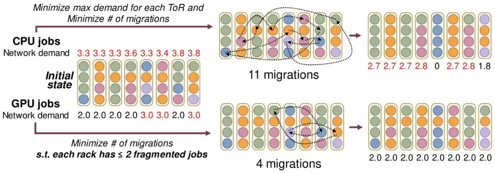
Diagram A. One replica group as its ring, ranks 0 to 11, each cell naming the worker's rack; red bars mark hops that leave a rack, and ↑ counts flows out of each rack. Ordered by rack (a), the ring leaves each rack once; interleaved (b), every hop crosses.圖解 A。把一個 replica group 畫成環，rank 0 到 11，每格標出 worker 所在的機櫃；紅條標出離開機櫃的跳，↑ 計算離開各機櫃的流數。依機櫃排序時（a），環對每個機櫃只離開一次；交錯排列時（b），每一跳都跨機櫃。Drawn for this primer from §3 of Zabreyko et al., SIGCOMM 2026 (arXiv 2602.08296v2).

Figure 2 of the paper shows why sparse ring traffic makes defragmentation tractable: five jobs on 32 servers in 8 racks need at least 11 migrations with CPU-style traffic, but 4 with GPU rings.

論文的 Figure 2 說明稀疏的環狀流量為何讓去碎片化變得可解：8 個機櫃、32 台伺服器上的五個任務，CPU 型流量至少需要 11 次遷移，GPU 環狀任務只需 4 次。

Figure 2 of the MonkeyTree paper: the same initial placement of five jobs on eight racks, migrated for CPU jobs (11 migrations, racks still above two units of demand) and for GPU ring jobs (4 migrations, every rack at 2.0) — Figure 2 of the paper, an illustration, not a measurement: colors are jobs, each ToR carries two units of demand, red values exceed it. After 11 CPU-style migrations (top) six racks remain over; after 4 GPU-aware migrations (bottom) every rack is at 2.0.論文的 Figure 2，是示意而非量測：顏色代表任務，每台 ToR 承載兩個單位的需求，紅色表示超過。CPU 型的 11 次遷移後（上）仍有六個機櫃超過；GPU 感知的 4 次遷移後（下）每個機櫃都是 2.0。Figure 2, Zabreyko, Wang and Ghobadi, "MonkeyTree: Near-Minimal Congestion for Multi-tenant Training via Migration", ACM SIGCOMM 2026 (arXiv 2602.08296v2).

3. The design3. 設計

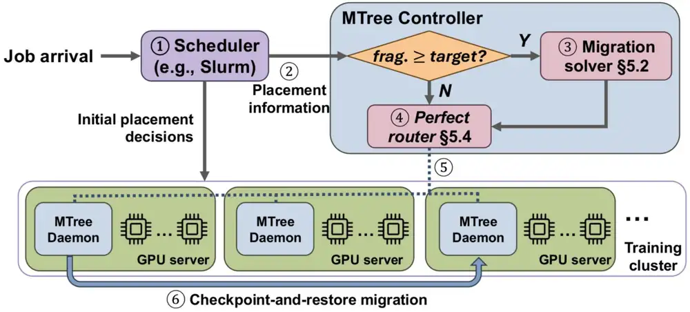
MonkeyTree runs beside the existing scheduler (Slurm in the paper) without changing how it allocates. If a rack's $f_t$ exceeds a threshold $\lambda$ , the uplinks per top-of-rack (ToR) switch, a controller solves for the fewest worker moves and routes every DP flow; per-node daemons carry out both. Three properties make this work: congestion-free placements are achievable, abundant and self-reinforcing.

MonkeyTree 與既有的排程器（論文中是 Slurm）並排運作，不改變它的分配方式。如果某個機櫃的 $f_t$ 超過門檻 $\lambda$ （每台機櫃頂端交換器 ToR 的上行數），控制器就求解最少的 worker 移動，並為每條 DP 流計算路由；每個節點的 daemon 執行兩者。三個性質讓這套做法成立：無壅塞的配置可達成、數量充足，而且會自我強化。

Figure 4 of the MonkeyTree paper: job arrival, the scheduler, the MonkeyTree controller with a fragmentation check, the migration solver and the Perfect router, daemons on GPU servers, and checkpoint-and-restore migration — Figure 4 of the paper, a design diagram: the scheduler places (1, 2), the controller plans moves only above the target (3), routes every DP flow (4), and daemons apply routes and migrate workers (5, 6).論文的 Figure 4，是設計示意圖：排程器配置（1、2），控制器只在超過目標時規劃移動（3）、為每條 DP 流計算路由（4），daemon 套用路由並遷移 worker（5、6）。Figure 4, Zabreyko, Wang and Ghobadi, "MonkeyTree: Near-Minimal Congestion for Multi-tenant Training via Migration", ACM SIGCOMM 2026 (arXiv 2602.08296v2).

3.1 Two uplinks are enough: Theorem 13.1 兩條上行就夠：定理 1

Theorem 1 states that for any cluster and any set of pure DP or FSDP jobs, some placement keeps every rack at $f_t \le 2$ . The proof is a construction. Order the jobs arbitrarily and fill the racks from left to right. Each rack then holds a front (the tail of a job from the previous rack), a middle (whole jobs) and an end (the head of a job that continues). Only the front and end jobs span racks, so $f_t \le 2$ (Diagram B, row b). The bound is tight: two jobs each larger than a rack, on three racks, share a rack that both span. With the routing of Section 3.3, two uplinks per rack suffice. Tensor parallelism changes the count, because each TP shard forms its own DP ring; with TP degree $D_C$ , Corollary 1 gives

定理 1 說：對任何叢集與任何一組純 DP 或 FSDP 任務，都存在讓每個機櫃 $f_t \le 2$ 的配置。證明是一個構造。把任務以任意順序排好，從左到右填滿機櫃。這樣每個機櫃有前段（來自前一個機櫃的任務尾巴）、中段（完整的任務）與末段（延續下去的任務開頭）。只有前段與末段的任務橫跨機櫃，所以 $f_t \le 2$ （圖解 B 的 b 列）。這個上限是緊的：兩個都比機櫃大的任務放在三個機櫃上時，必然共用一個兩者都橫跨的機櫃。搭配第 3.3 節的路由，每個機櫃兩條上行就夠。張量平行會改變計數，因為每個 TP 分片各自組成一個 DP 環；TP 度數為 $D_C$ 時，推論 1 給出

f_t \le 2\,D_C

so with TP 8 on 8-GPU servers, a rack needs at least 16 uplinks.

所以在 8 顆 GPU 的伺服器上使用 TP 8 時，一個機櫃至少需要 16 條上行。

Diagram B. Four DP jobs (A 10, B 6, C 7, D 5 workers) on racks of 8 slots;

f

is each rack's fragmentation degree, red above

\lambda = 2

, and

\Delta

counts moves from row a. (a) A scheduler placement after churn. (b) Theorem 1's fill. (c) The integer program's choice; bold cells moved.圖解 B。四個 DP 任務（A 10、B 6、C 7、D 5 個 worker）在各 8 格的機櫃上；

f

是各機櫃的碎片化度數，超過

\lambda = 2

時標紅，

\Delta

是距 a 列的移動次數。(a) 任務來去後排程器的配置。(b) 定理 1 的填法。(c) 整數規劃的選擇；粗框是移動過的格子。Drawn for this primer from §5.1–§5.2 of Zabreyko et al.; the placements and move counts are our own example, computed with the paper's objective.

3.2 The fewest moves: a small integer program3.2 最少的移動：一個小型整數規劃

The solver takes the current placement $w_0(s,t)$ , the workers of job $s$ on rack $t$ , plus job sizes $s_j$ , rack capacity $C$ and $\lambda$ , and returns the placement $w(s,t)$ that moves the fewest workers, subject to job sizes, capacity and the bound:

求解器輸入目前的配置 $w_0(s,t)$ （任務 $s$ 在機櫃 $t$ 上的 worker 數），加上任務大小 $s_j$ 、機櫃容量 $C$ 與 $\lambda$ ，輸出在任務大小、容量與上限的限制下，移動 worker 最少的配置 $w(s,t)$ ：

\min_{w}\ \tfrac12 \sum_{s,t} \big|\,w(s,t) - w_0(s,t)\,\big|

\begin{gathered} \textstyle\sum_{t} w(s,t) = s_j, \qquad \sum_{s} w(s,t) \le C, \\ f_t(w) \le \lambda, \qquad w(s,t) \in \mathbb{Z}_{\ge 0} \end{gathered}

\begin{gathered} f_t(w) = |S_t|, \\ S_t = \{\, s : w(s,t) > 0 \ \wedge\ \textstyle\sum_{t' \ne t} w(s,t') > 0 \,\} \end{gathered}

The half turns a distance into a move count, because one move lowers one entry and raises another. The problem, a variant of the sparsity-constrained transport problem, is NP-hard. Branch-and-bound still solves it exactly: it drops every branch that already needs as many moves as the best solution found, and only $O(N^{2\gamma})$ placements of $N$ nodes lie within $\gamma$ moves. Answers stay small because compliance is self-reinforcing: a new job touches only the racks where the scheduler put it. Pipeline stages count as separate jobs, TP jobs are weighted by their ring count $d_s$ , and expert parallelism gets no guarantee.

這個二分之一把距離換成移動次數，因為一次移動讓一個項目減一、另一個加一。這個問題是稀疏度受限運輸問題的變形，屬於 NP-hard。branch-and-bound 仍能精確求解：它丟棄所有已需要與目前最佳解一樣多移動的分支，而 $N$ 個節點時， $\gamma$ 次移動內只有 $O(N^{2\gamma})$ 個配置。答案保持很小，是因為符合條件的狀態會自我強化：新任務只碰到排程器放它的那幾個機櫃。管線階段被當成獨立的任務，TP 任務以環數 $d_s$ 加權，專家平行則沒有保證。

Diagram C. The panel's default; ↑1 and ↑2 list the jobs whose ring flow leaves on each uplink. (a) R3 holds three fragmented jobs, so A and C share ↑1 whatever the routing does. (b) After C's two workers move to R4, every flow is isolated.圖解 C。面板的預設情境；↑1 與 ↑2 列出從各條上行離開的任務環流。(a) R3 有三個碎片化任務，所以不論路由怎麼做，A 與 C 都得共用 ↑1。(b) C 的兩個 worker 移到 R4 後，每條流都被隔離。Drawn for this primer with the paper's objective (§5.2) and Perfect routing (§5.4); the uplink labels come from one valid coloring of these ring flows.

Panel 1面板 1

Place and migrate workers on four racks在四個機櫃上配置與遷移 worker

Data-parallel jobs資料平行任務數

Uplinks per rack, threshold

\lambda

每個機櫃的上行數，門檻

\lambda

Placement配置

Fragmentation degree, R1 to R4

碎片化度數，R1 到 R4

Racks over

\lambda

超過

\lambda

的機櫃

Most jobs on one uplink

單條上行上最多的任務數

Moves made

已做的移動

Fewest moves to comply

達成條件的最少移動

Pause from your moves

你的移動造成的暫停

Each slot is one worker of a pure data-parallel job, and each job's ring visits its racks in order, so a rack sends one flow out per fragmented job. Click a worker, then a free slot to move it, or another job's worker to swap the two (2 moves). "Scheduler placement" restores a placement left by churn; "Sequential fill" applies Theorem 1's construction; "Fewest moves" solves the integer program of Section 3.2 by branch-and-bound over per-rack counts. The uplink boxes come from Perfect routing: a bipartite edge coloring of the ring flows, folded round-robin onto $\lambda$ uplinks when colors exceed $\lambda$ , as in the paper's fallback. The pause per moved worker is the prototype's measured 9.02 s overhead plus 1.07 s on the wire (Llama3-8B, 12 GB shard, A100 with a 100 Gb/s ConnectX-5); we sum it over moved workers and do not scale it to other models. Defaults: three jobs and two uplinks per rack, as in the paper's Figure 2 toy. Try four jobs at $\lambda = 1$ , then at $\lambda = 3$ .

每一格是一個純資料平行任務的 worker，每個任務的環依序走過它的機櫃，所以每個碎片化任務從一個機櫃送出一條流。點一個 worker，再點空格就能移動它；點另一個任務的 worker 則兩者互換（2 次移動）。「排程器的配置」還原任務來去後留下的配置；「依序填入」套用定理 1 的構造；「最少移動」以 branch-and-bound 在各機櫃的計數上求解第 3.2 節的整數規劃。上行方塊來自 Perfect routing：對環流做二分圖邊著色，顏色多於 $\lambda$ 時依論文的備案輪流折疊到 $\lambda$ 條上行上。每個被移動 worker 的暫停時間是原型實測的 9.02 s 開銷加上線路上的 1.07 s（Llama3-8B、12 GB 分片、A100 搭配 100 Gb/s ConnectX-5）；我們把它對被移動的 worker 加總，並不換算到其他模型。預設值：三個任務、每個機櫃兩條上行，與論文 Figure 2 的小例子相同。試試四個任務在 $\lambda = 1$ ，再試 $\lambda = 3$ 。

Stop and think停下來想一想

With four jobs at $\lambda = 2$ , compare the moves of "Sequential fill" and "Fewest moves". Both comply; why not use Theorem 1's construction? Then try $\lambda = 3$ and $\lambda = 1$ .

四個任務、 $\lambda = 2$ 時，比較「依序填入」與「最少移動」的移動次數。兩者都符合條件；為何不用定理 1 的構造？接著試 $\lambda = 3$ 與 $\lambda = 1$ 。

3.3 Then routing is easy: Perfect routing3.3 接著路由就容易了：Perfect routing

With $f_t \le \lambda$ on every rack, each DP flow gets its own uplink. The cross-rack flows form a bipartite multigraph from sending to receiving racks. Color its edges so that no rack has two edges of one color, one color per spine. By König's theorem the colors needed equal the largest degree, at most $\lambda$ , and repeated Hopcroft–Karp matching finds them in polynomial time. Daemons pick header values whose ECMP hash lands on the assigned uplink. Without migration, extra colors fold onto uplinks round-robin; small non-DP flows such as PP go round-robin over the spines.

每個機櫃都滿足 $f_t \le \lambda$ 時，每條 DP 流都有自己的上行。跨機櫃的流構成從送出機櫃到接收機櫃的二分多重圖。替它的邊著色，讓同一個機櫃沒有兩條同色的邊，每種顏色對應一台 spine。依 König 定理，所需顏色數等於最大度數，最多是 $\lambda$ ；反覆以 Hopcroft–Karp 求匹配，可在多項式時間內找出著色。daemon 選擇讓 ECMP 雜湊落在指定上行的標頭值。不做遷移時，多出的顏色輪流折疊到上行上；PP 這類小的非 DP 流則輪流分配到各台 spine。

Where Crux fits. MonkeyTree decides where workers sit, which bounds the flows per rack. Crux decides, on a given placement, which path each flow takes and which job waits when flows meet. So they compose: in the paper's MonkeyTree-Crux variant, Crux's routing replaces Perfect routing on MonkeyTree's placements. On a bounded placement an isolated assignment exists; on an unbounded one, scheduling can only choose who suffers. The paper's Crux is greedy routing without priority levels, and the comparison is simulated, so we quote no numbers.

Crux 的位置。MonkeyTree 決定 worker 坐在哪裡，因而限制每個機櫃的流數。Crux 則在給定的配置上，決定每條流走哪條路徑、流相遇時哪個任務等待。所以兩者可以組合：在論文的 MonkeyTree-Crux 變形中，Crux 的路由取代 Perfect routing，疊在 MonkeyTree 的配置上。在有上限的配置上，一定存在互相隔離的指派；在沒有上限的配置上，排程只能選擇誰受害。論文中的 Crux 是沒有優先權層級的貪婪路由，而且比較是模擬的，所以我們不引用數字。

3.4 Moving a worker: checkpoint and restore over RDMA3.4 移動一個 worker：透過 RDMA 的檢查點與還原

A move is an in-memory checkpoint and restore. The source pauses after its iteration, so the whole job waits, and writes model and optimizer state by GPUDirect RDMA into CPU memory on a staging server. The destination loads it, starts NCCL and rejoins its replica group. Jobs start with ring orders computed in advance; the paper does not say how, but Diagram A shows that each rack's workers must stay adjacent.

一次移動就是記憶體內的檢查點與還原。來源在迭代結束後暫停，所以整個任務都在等；它以 GPUDirect RDMA 把模型與最佳化器狀態寫進暫存伺服器的 CPU 記憶體。目的端載入狀態、啟動 NCCL，再回到它的 replica group。任務以事先算好的環順序啟動；論文沒有說明怎麼算，但圖解 A 顯示同一機櫃的 worker 必須保持相鄰。

4. Implementation4. 實作

The simulator is about 20,000 lines of Rust with a max-min flow-level network model; each simulated migration costs a barrier, a shard transfer and a 10 s pause taken from the prototype. The prototype extends PyTorch Distributed Checkpoint with RDMA StorageReader and StorageWriter classes, and its controller talks to Slurm. It runs on five servers, each with one A100 GPU and one 100 Gb/s ConnectX-5 NIC. The paper gives no line count and promises the code at publication.

模擬器約 20,000 行 Rust，網路使用 max-min 流級模型；每次模擬的遷移代價是一個屏障、一次分片傳輸，以及取自原型的 10 s 暫停。原型以 RDMA 的 StorageReader 與 StorageWriter 類別擴充 PyTorch Distributed Checkpoint，控制器與 Slurm 溝通。它跑在五台伺服器上，每台一顆 A100 GPU 與一張 100 Gb/s ConnectX-5 NIC。論文沒有給出程式行數，並承諾在發表時公開程式碼。

5. What was measured5. 量到了什麼

Two kinds of numbers are measured. Slowdown, completion time, fragmentation over time, moves per event and migration durations all come from the simulator, with up to 2,048 simulated H200-class GPUs, so we leave them out.

實測的數字只有兩類。減速、完成時間、碎片化隨時間的變化、每次事件的移動數與遷移時長，都來自最多模擬 2,048 顆 H200 級 GPU 的模擬器，所以我們不列入。

One move (Figure 13 of the paper). On a four-node Llama3-8B job, one worker moved a 12 GB shard of weights and optimizer state. Composing the checkpoint took 3.93 s. The RDMA transfer took 3.19 s, of which only 1.07 s was on the wire at about 90 Gb/s; the rest was serialization and memory management. Destination startup took 2.97 s, and source cleanup, 1.24 s, ran in the background. The overhead without network time is 9.02 s.

一次移動（論文 Figure 13）。在一個四節點的 Llama3-8B 任務上，移動一個 worker，帶著 12 GB 的權重與最佳化器狀態分片。組合檢查點花了 3.93 s。RDMA 傳輸花了 3.19 s，其中只有 1.07 s 以約 90 Gb/s 在線路上；其餘是序列化與記憶體管理。目的端啟動花了 2.97 s，來源端 1.24 s 的清理在背景執行。扣除網路時間後的開銷是 9.02 s。

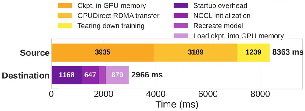
Figure 13 of the MonkeyTree paper: stacked bars of migration phases in milliseconds, source 3,935 checkpoint, 3,189 RDMA transfer, 1,239 teardown (8,363 total); destination startup, NCCL initialization, model recreation and checkpoint load (2,966 total) — Figure 13 of the paper, measured on the A100 and ConnectX-5 testbed for one Llama3-8B worker; each side starts at zero. The network is a small part of the cost.論文的 Figure 13，在 A100 與 ConnectX-5 測試平台上針對一個 Llama3-8B worker 實測；兩側都從零開始。網路只占成本的一小部分。Figure 13, Zabreyko, Wang and Ghobadi, "MonkeyTree: Near-Minimal Congestion for Multi-tenant Training via Migration", ACM SIGCOMM 2026 (arXiv 2602.08296v2).

Drawn as one timeline, with the three blocking phases in sequence:

畫成一條時間軸，三個會擋住任務的階段依序排列：

Diagram D. The measured timeline of one migration, in which the darker part of the transfer marks the 1.07 s spent on the wire, drawn at the end of the transfer, while the grey box at the source is the cleanup that runs in the background.圖解 D。一次遷移的實測時間軸，傳輸中顏色較深的部分代表線路上的 1.07 s，畫在傳輸的末段，而來源端的灰色框則是在背景執行的清理。Drawn for this primer from §7 and Figure 13 of Zabreyko et al.

In that order the parts add up exactly to the overhead plus the wire time:

依此順序，各部分相加正好等於開銷加上線路時間：

Question問題	Calculation算式	Result結果
Blocking phases: compose, transfer, destination startup會擋住任務的階段：組合、傳輸、目的端啟動	$3.93 + 3.19 + 2.97$	$\approx 10.09$ s
Without the time on the wire扣除線路上的時間	$10.09 - 1.07$	$9.02$ sthe paper's overhead即論文報告的開銷
Check the wire time: 12 GB at about 90 Gb/s驗算線路時間：12 GB、約 90 Gb/s	$12 \times 8 \div 90$	$\approx 1.07$ s
Share of a move spent on the wire一次移動中花在線路上的比例	$1.07 \div 10.09$	$\approx 11\%$

So a move pauses its job for about 10 s, the pause the simulator assumes, and a faster NIC would barely help.

所以一次移動會讓它的任務停約 10 s，正是模擬器假設的暫停時間；換更快的 NIC 幫助不大。

Solver run time (Figures 9 and 10 of the paper). The run times are measured, on cluster states that the simulator produced. The paper does not name the machine or the solver product.

求解器執行時間（論文 Figures 9 與 10）。執行時間是實測的，量測對象是模擬器產生的叢集狀態。論文沒有指明機器或求解器產品。

Cluster叢集	Case情況	Measured solve time實測求解時間
1,024 GPUs1,024 顆 GPU	2-move solutions需 2 次移動的解	540 ms average, never above 4 s平均 540 ms，從未超過 4 s
1,024 GPUs1,024 顆 GPU	6-move solutions需 6 次移動的解	6.7 s, roughly linear in moves6.7 s，大致隨移動數線性成長
Up to 1,024 GPUs最多 1,024 顆 GPU	All events所有事件	Under 0.5 s average, p90 under 1 s平均低於 0.5 s，p90 低於 1 s
2,048 GPUs2,048 顆 GPU	All events所有事件	2.39 s average, 4.04 s p90平均 2.39 s，p90 為 4.04 s

The time grows more than fivefold from 1,024 to 2,048 GPUs, which is why the paper proposes partitions for larger clusters.

從 1,024 到 2,048 顆 GPU，時間成長超過五倍，這就是論文為更大的叢集提出分區的原因。

6. Limits and open questions6. 限制與未解的問題

The paper's own limits: larger clusters need partitions under a second-tier controller; three-tier and rail-optimized fabrics are sketched, not evaluated; expert parallelism's all-to-all can rival DP, and context parallelism puts each node in two rings, an NP-hard min-cut variant, so neither gets a guarantee. A careful reader adds:

論文自己的限制：更大的叢集需要由第二層控制器管理的分區；三層網路與 rail-optimized 網路只有構想，沒有評估。專家平行的 all-to-all 流量可與 DP 相當，上下文平行讓每個節點同時在兩個環上（NP-hard 的最小割變形），所以兩者都沒有保證。細心的讀者還應該補上：

Rings. NCCL also uses trees, PAT and NVLS, and several channels per communicator, each its own ring; channels multiply the flows per rack as TP does.環。NCCL 也會用 tree、PAT 與 NVLS，而且每個 communicator 有好幾個 channel，各是一個環；channel 會像 TP 一樣讓每個機櫃的流數倍增。
Evidence. The system results come from a flow-level simulator without PFC, DCQCN or buffers; Wormhole measured about 20% flow-completion-time error for a flow-level simulator against ns-3 on LLM training traffic.證據。系統層級的結果來自沒有 PFC、DCQCN 與緩衝的流級模擬器；Wormhole 在 LLM 訓練流量上，量到流級模擬器相對 ns-3 約 20% 的流完成時間誤差。
One cost point. An 8B model, a 12 GB shard, single-GPU nodes; whole servers and failures during a move are unmeasured.只有一個代價點。8B 模型、12 GB 分片、單 GPU 節點；整台伺服器與移動途中的故障都沒有量測。
Path control and status. Perfect routing needs the switches' ECMP hash functions, as Crux and HPN do. The code is unreleased and no production use is reported.路徑控制與現況。Perfect routing 需要知道交換器的 ECMP 雜湊函數，Crux 與 HPN 也一樣。程式碼尚未公開，也沒有回報生產使用。

7. How it connects7. 與其他內容的關聯

Chapter 11, sections 2 and 3: "order the ring pod by pod" becomes a per-rack count with a guarantee, and defragmentation becomes continuous, at about 10 s per moved worker.第 11 章第 2 與第 3 節：「依 pod 排序環」變成有保證的逐機櫃計數，去碎片化也變成持續的流程，每移動一個 worker 約 10 s。
Crux and LEVELLER ration the contention a placement leaves; SimAI and Wormhole could test MonkeyTree at packet level.Crux 與 LEVELLER 分配配置所留下的競爭；SimAI 與 Wormhole 可以在封包層級檢驗 MonkeyTree。
Alibaba HPN moved a job of more than 2,300 GPUs from 19 segments to 3 and measured 14.9% more throughput: production evidence that defragmenting pays. Meta's minimum-cut placement and Llama 3's [TP, CP, PP, DP] order are static versions of the idea; Rail-only, from the same MIT group, motivates the per-rail extension.Alibaba HPN 把一個超過 2,300 顆 GPU 的任務從 19 個 segment 搬到 3 個，量到吞吐提升 14.9%：這是去碎片化值得的生產證據。Meta 的最小割配置與 Llama 3 的 [TP, CP, PP, DP] 順序是這個想法的靜態版本；來自同一個 MIT 團隊的 Rail-only 則是逐 rail 延伸的動機。

Key numbers關鍵數字

Number	數字	Meaning and setup
9.02 s	Overhead of one move without 1.07 s on the wire (Llama3-8B, 12 GB shard, A100 + 100 Gb/s ConnectX-5)	一次移動的開銷，不含線路上的 1.07 s（Llama3-8B、12 GB 分片、A100 + 100 Gb/s ConnectX-5）
3.93 / 3.19 / 2.97 s	Compose / RDMA transfer / destination startup (same prototype)	組合 / RDMA 傳輸 / 目的端啟動（同一原型）
540 ms	Average solve time of 2-move solutions at 1,024 GPUs (run time measured on simulated states)	1,024 顆 GPU 時需 2 次移動之解的平均求解時間（在模擬狀態上實測的執行時間）
2.39 s / 4.04 s	Average / p90 solve time at 2,048 GPUs (same method)	2,048 顆 GPU 時的平均 / p90 求解時間（同一方法）
$f_t \le 2$ ; $2D_C$	Bound for pure DP or FSDP (Theorem 1); with TP degree $D_C$ (Corollary 1); analysis	純 DP 或 FSDP 的上限（定理 1）；TP 度數為 $D_C$ 時（推論 1）；分析結果
840 GB / 48 GB	DP / PP bytes per iteration, Llama3-70B, 128 GPUs (Table 1, analysis)	Llama3-70B、128 顆 GPU 每次迭代的 DP / PP 位元組（Table 1，分析）

Terms used on this page本頁用到的術語

Fragmentation degree: The DP flows that leave a rack; for pure DP jobs, the jobs with workers both inside and outside it.; 離開一個機櫃的 DP 流數；對純 DP 任務，就是在機櫃內外都有 worker 的任務數。
Perfect routing: One uplink per cross-rack DP flow, found by a bipartite edge coloring of the flows.; 以流的二分圖邊著色，讓每條跨機櫃 DP 流各有一條上行。
Branch-and-bound: An exact search that drops every branch already worse than the best solution found.; 一種精確搜尋，丟棄所有已比目前最佳解更差的分支。
Max-min flow-level simulator: A simulator that gives each flow its fair share of every link, with no packets, queues or congestion control.; 讓每條流在每條鏈路上取得公平份額的模擬器，沒有封包、佇列或壅塞控制。