Research digest 1 of 5 · Chapter 11: Sharing the cluster

研究導讀 1 / 5 · 第 11 章：共用叢集

Crux: GPU-Efficient Communication Scheduling for Deep Learning TrainingCrux：以 GPU 效率為目標的深度學習訓練通訊排程

SIGCOMM 2024Jiamin Cao, Yu Guan, Kun Qian et al. (Alibaba Cloud) · paper論文

After reading, you can explain how Crux decides whose traffic goes first on a shared link: GPU intensity, path choice, corrected priorities, and compression into a few switch queues.讀完後，你能說明 Crux 如何決定共享鏈路上誰的流量先走：GPU 強度、路徑選擇、修正後的優先權，以及壓縮到少數交換器佇列。

≈ 11 min · 1 interactive panel · 5-question quiz≈ 11 分鐘 · 1 個互動面板 · 5 題測驗Chapter 11 ↗第 11 章 ↗Jump to the quiz ↓跳到測驗 ↓

If you read nothing else

只讀這一段也可以

In Alibaba's two-week trace of a shared cluster with more than 2,000 GPUs, 36.3% of jobs, holding 51% of the GPUs, were exposed to link contention with other jobs, mostly through ECMP hash collisions. That number counts exposure, not measured slowdown. One measured pair shows the cost: next to a BERT job, a 64-GPU GPT job slowed from 1.53 s to 1.70 s per iteration, and GPU utilization fell 9.5%. Crux ranks jobs by GPU intensity, computation per iteration over bottleneck communication time, and uses the rank to pick ECMP paths and fill about 8 switch priority levels. On 96 GPUs it raised utilization by 8.3–14.8%; the favored job's JCT fell by up to 33%, the others' rose by at most 3%.

在阿里對一座超過 2,000 顆 GPU 的共享叢集所做的兩週追蹤中，36.3% 的任務（占 51% 的 GPU）曝露於與其他任務的鏈路競爭，主要來自 ECMP 雜湊碰撞。這個數字算的是曝露，不是量到的變慢。一組實測的任務對顯示了代價：與一個 BERT 任務並存時，64 顆 GPU 的 GPT 任務每次迭代從 1.53 s 變成 1.70 s，GPU 使用率下降 9.5%。Crux 依 GPU 強度（每次迭代的計算量除以瓶頸通訊時間）為任務排序，並用這個排名選擇 ECMP 路徑、填入約 8 個交換器優先權等級。在 96 顆 GPU 上，它讓使用率提高 8.3–14.8%；受優待任務的 JCT 最多縮短 33%，其他任務的 JCT 最多增加 3%。

1. Where this paper sits1. 這篇論文的位置

Section 11.1 ("What one job does to another") lists three ways one job slows another: hash collisions, PFC pauses and unequal cost. For the third it quotes Crux's rule: give the link to the job whose waiting GPUs are worth the most. The rule needs a number for the worth of traffic, a way to act on a commodity RoCE fabric, and a way to fit thousands of jobs into about 8 priority levels. Earlier schedulers miss at least one. Varys and Sincronia ignore computation, TACCL ignores other jobs, and CASSINI shifts jobs in time instead of ranking them.

第 11.1 節（「一個任務對另一個任務做了什麼」）列出一個任務拖慢另一個任務的三種方式：雜湊碰撞、PFC 暫停與代價不對等。對第三種，它引用 Crux 的規則：把鏈路交給等待中 GPU 價值最高的任務。這條規則需要一個衡量流量價值的數字、在商用 RoCE 網路上執行它的方法，以及把數千個任務塞進約 8 個優先權等級的方法。先前的排程器至少缺一樣。Varys 與 Sincronia 忽略計算，TACCL 忽略其他任務，CASSINI 在時間上錯開任務而不是為它們排名。

2. The problem, measured2. 問題，用量測說話

The trace covers two weeks of August 2023: more than 2,000 GPUs, a three-layer Clos, more than 5,000 jobs, and more than 30 jobs at once at peak. The paper says that 36.3% of jobs, holding 51% of the GPUs, "may suffer communication contention". The number comes from placement and topology. It counts jobs whose traffic could share a link; it does not measure a slowdown. Most exposure is on network paths (ECMP hash collisions); a minority is on PCIe inside hosts (fragmented GPU allocation).

追蹤涵蓋 2023 年 8 月的兩週：超過 2,000 顆 GPU、三層 Clos、超過 5,000 個任務，尖峰時有超過 30 個任務同時執行。論文說 36.3% 的任務（占 51% 的 GPU）「可能遭遇通訊競爭」。這個數字來自配置與拓樸。它算的是流量可能共用某條鏈路的任務；它沒有量測變慢多少。大部分曝露在網路路徑上（ECMP 雜湊碰撞）；少部分在主機內的 PCIe 上（GPU 配置碎片化）。

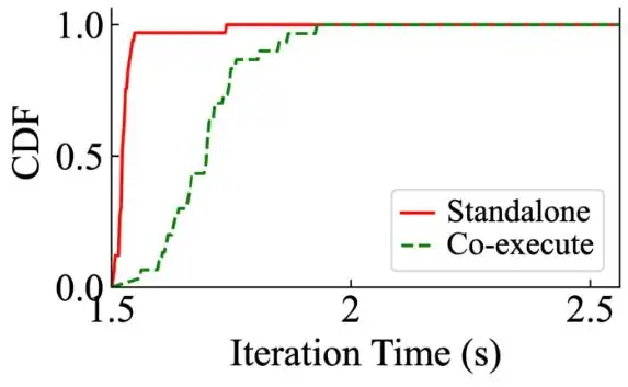
To measure the cost, the authors re-ran a representative contending pair from the production cluster. A 64-GPU GPT job (a GPT-3 variant cut to 24 layers) ran on 8 hosts and a 16-GPU BERT job on 4 hosts, under the same two ToR switches; they met on the ToR–aggregation links. GPT's iteration time rose 11.0%, from 1.53 s to 1.70 s (the paper's Figure 7, below). Throughput fell 9.9% for GPT and 7.7% for BERT, and GPU utilization 9.5%, because GPT holds four times BERT's GPUs.

為了量出代價，作者重新執行從生產叢集取樣的一組有代表性的競爭任務。64 顆 GPU 的 GPT 任務（縮減為 24 層的 GPT-3 變體）跑在 8 台主機上，16 顆 GPU 的 BERT 任務跑在 4 台主機上，都在同樣兩台 ToR 交換器之下；它們在 ToR 到聚合層的鏈路上相遇。GPT 的迭代時間增加 11.0%，從 1.53 s 變成 1.70 s（論文圖 7，見下圖）。GPT 的吞吐下降 9.9%、BERT 下降 7.7%，GPU 使用率下降 9.5%，因為 GPT 的 GPU 是 BERT 的四倍。

CDF of GPT iteration time: standalone runs near 1.53 s, co-executed runs spread from about 1.55 to 1.9 s — Figure 7 of the paper: the CDF of GPT's iteration time when it runs alone (red, solid) and next to the BERT job (green, dashed), measured in the authors' cluster. The whole distribution shifts to the right.論文圖 7：GPT 單獨執行（紅色實線）與和 BERT 任務並存（綠色虛線）時迭代時間的 CDF，於作者的叢集實測。整個分布都往右移。Cao et al., SIGCOMM 2024, Figure 7 (measured re-run of a production job pair).

The paper converts the loss into machines and money:

論文把損失換算成機器與金錢：

Question問題	Calculation算式	Result結果
GPUs lost in a 1,000-GPU cluster at −9.5%1,000 顆 GPU 的叢集在 −9.5% 時損失的 GPU	$1{,}000 \times 0.095$	95 GPUs95 顆 GPU
10% of 10,000 GPUs, at about $40 per 8-GPU server-hour10,000 顆 GPU 的 10%，每台 8-GPU 伺服器每小時約 $40	$0.1 \times 10{,}000 \div 8 \times 40 \times 24$	$120,000 per day每天 $120,000

Why utilization, not average job completion time (JCT)? In the paper's Figure 8 (shown in Chapter 11), both orders of a 1-GPU and a 10-GPU job give the same average JCT, but one idles 10 GPUs and the other 1.

為什麼看使用率，而不是平均任務完成時間（JCT）？在論文 Figure 8（第 11 章有附）中，1 顆 GPU 與 10 顆 GPU 的任務不論哪個先走，平均 JCT 都相同，但一種讓 10 顆 GPU 閒著，另一種只讓 1 顆閒著。

3. The design3. 設計

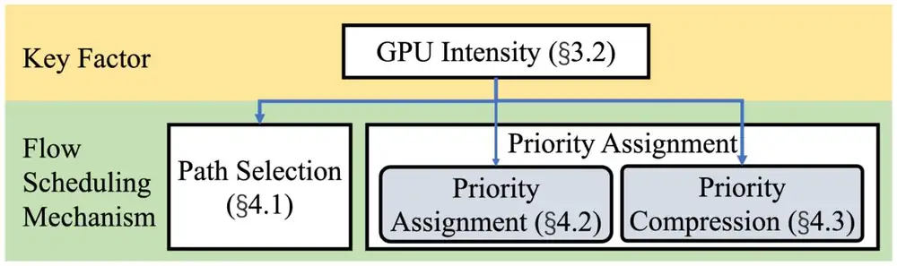
The paper models GPUs as nodes and links (network and PCIe) as edges with bandwidth $B_e$ . Job $j$ computes $W_j$ per iteration and sends $M_{j,e}$ bytes over link $e$ . Three mechanisms act on this model: path selection, priority assignment and priority compression. The paper's Figure 10 (below) shows that all three take GPU intensity as their input.

論文把 GPU 建模為節點，把鏈路（網路與 PCIe）建模為頻寬 $B_e$ 的邊。任務 $j$ 每次迭代計算 $W_j$ ，並在鏈路 $e$ 上送 $M_{j,e}$ 位元組。三個機制作用在這個模型上：路徑選擇、優先權指派與優先權壓縮。論文圖 10（見下圖）顯示這三者都以 GPU 強度為輸入。

Block diagram: GPU Intensity (§3.2) in a yellow Key Factor band, with arrows down to Path Selection (§4.1) and to Priority Assignment (§4.2) and Priority Compression (§4.3) in a green Flow Scheduling Mechanism band. — Figure 10 of the paper: the overview of Crux (a design diagram). GPU intensity, the key factor (the paper's §3.2), feeds path selection (§4.1) and priority assignment, which has two parts: assigning priorities (§4.2) and compressing them into the few hardware levels (§4.3). On this page these are sections 3.1 to 3.4.論文圖 10：Crux 的總覽（設計示意圖）。關鍵因素 GPU 強度（論文 §3.2）供給路徑選擇（§4.1）與優先權指派；後者分成兩部分：指派優先權（§4.2），以及把優先權壓縮進少數硬體等級（§4.3）。在本頁，它們是第 3.1 到 3.4 節。Cao et al., SIGCOMM 2024, Figure 10 (author PDF, p. 5, re-rendered).

3.1 GPU intensity: what a byte is worth3.1 GPU 強度：一個位元組值多少

Utilization over a period $T$ is the work that all GPUs complete, $U_T = \sum_v L_v$ . Crux values a job's traffic by its GPU intensity:

一段時間 $T$ 內的使用率是所有 GPU 完成的工作量， $U_T = \sum_v L_v$ 。Crux 以任務的 GPU 強度（GPU intensity）衡量其流量的價值：

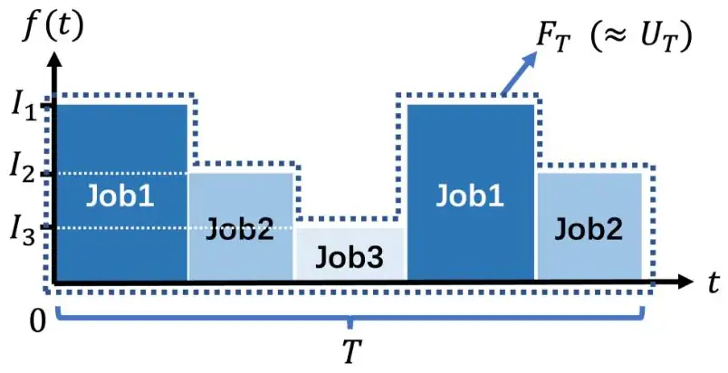
I_j = \frac{W_j}{t_j}, \qquad t_j = \max_{e} \frac{M_{j,e}}{B_e}

$t_j$ is the time that the job's traffic needs on its slowest link, so $I_j$ is the computation unblocked per second of bottleneck communication. On one link, let $F_T$ be the integral over time of the intensity of whichever job occupies the link (the paper's Figure 9, below). Theorem 1 states that F_T/U_T tends to 1 as T grows, under the proof's conditions: the same pairing repeats across iterations, the set of jobs is fixed and finite, and there is one bottleneck link. The proof is in Appendix A. The main text concludes: keep the link busy with the most intensive traffic. It also argues that one bottleneck link per job is enough, and that the full problem is NP-complete.

$t_j$ 是任務流量在最慢鏈路上需要的時間，所以 $I_j$ 是每秒瓶頸通訊所解開的計算量。在單一鏈路上，令 $F_T$ 為「占用鏈路之任務的強度」對時間的積分（論文圖 9，見下圖）。Theorem 1 說：在證明的前提下（每輪迭代重複同樣的配對、任務集合固定且有限、只有一條瓶頸鏈路），T 變大時 F_T/U_T 趨近 1。證明在附錄 A。正文的結論是：讓鏈路一直忙著傳最密集的流量。正文也主張每個任務只需考慮一條瓶頸鏈路，而且完整的問題是 NP-complete。

Step chart f(t): rectangles for Job1, Job2 and Job3 at heights I1, I2 and I3 over a period T, with the total area labelled F_T — Figure 9 of the paper: the jobs that occupy one link over a period $T$ (a model illustration, not data). Each block is one transfer; its width is the transmission time and its height the job's intensity $I_j$ . The paper labels the total area $F_T$ as tracking utilization $U_T$ .論文圖 9：一段時間 $T$ 內占用一條鏈路的任務（模型示意圖，不是資料）。每個方塊是一次傳輸；寬度是傳輸時間，高度是任務的強度 $I_j$ 。論文把總面積 $F_T$ 標為追蹤使用率 $U_T$ 。Cao et al., SIGCOMM 2024, Figure 9 (design illustration).

3.2 Path selection by intensity3.2 依強度選擇路徑

A collision between two intensive jobs costs the most. So Crux sorts jobs by intensity, and each job in turn takes the least-congested path that remains, recomputed when a job arrives or ends; a low-intensity job that still collides loses priority anyway. Crux finds the ECMP paths by probing with different UDP source ports (INT records the hops) and pins one port per queue pair with ibv_modify_qp.

兩個密集任務之間的碰撞代價最高。所以 Crux 依強度排序任務，每個任務依序取剩下最不壅塞的路徑，任務到達或結束時重新計算；仍然碰撞的低強度任務反正會失去優先權。Crux 以不同的 UDP 來源埠送出探測封包來找出 ECMP 路徑（INT 記錄經過的每一跳），再用 ibv_modify_qp 為每個 queue pair 固定一個來源埠。

3.3 Priority assignment with corrections3.3 帶修正的優先權指派

Where contention remains, strict priority decides who sends. Intensity alone is not enough. In the paper's Example 1 (Diagram A), two 10-GPU jobs have equal intensity, 5 Gflops per second of communication. Job 1 computes 2 s and sends 2 s per iteration; Job 2 computes 1 s and sends 1 s. Job 1 first gives 37.5% utilization; Job 2 first gives 41.7%. Example 2 adds overlap: a job whose communication hides behind its own computation loses nothing when delayed, so the other job should go first.

競爭仍在之處，由嚴格優先權決定誰先送。只看強度不夠。在論文的 Example 1（示意圖 A）中，兩個 10 顆 GPU 的任務強度相同，每秒通訊對應 5 Gflops。任務 1 每次迭代計算 2 s、傳送 2 s；任務 2 計算 1 s、傳送 1 s。任務 1 優先得到 37.5% 的使用率；任務 2 優先得到 41.7%。Example 2 加入重疊：通訊藏在自己計算後面的任務，被延遲也沒有損失，所以應該讓另一個任務先走。

Diagram A. Example 1 (the paper's Figure 11) over 12 s of steady state. GPUs idle while their job sends or waits. With Job 2 first, Job 2 gains 3 iterations and Job 1 loses 1.示意圖 A。Example 1（論文 Figure 11）穩態下的 12 s。任務傳送或等待時，它的 GPU 閒置。任務 2 優先時，任務 2 多 3 次迭代，任務 1 少 1 次。Drawn for this primer from Cao et al., SIGCOMM 2024, §4.2 and Figure 11 (worked example); timelines from our fluid model of one link, which reproduces both stated utilizations.

So Crux uses $P_j = k_j\, I_j$ . The reference job, the one with the most traffic, has $k = 1$ . For each other job, Crux replays both orders against it on a per-iteration timeline and finds the intensity ratio at which they tie. For Example 1:

所以 Crux 使用 $P_j = k_j\, I_j$ 。參考任務（流量最多的任務）的 $k = 1$ 。對其他每個任務，Crux 在每次迭代的時間軸上重演它與參考任務的兩種順序，找出兩者打平時的強度比。以 Example 1 為例：

Question問題	Calculation算式	Result結果
Link seconds per 12 s (Job 1, Job 2): Job 1 first; Job 2 first每 12 s 的鏈路秒數（任務 1、任務 2）：任務 1 優先；任務 2 優先	$(6, 3);\ (4, 6)$	from the paper取自論文
What each order gains for its own job每種順序為自己的任務多得的時間	$6 - 4;\ 6 - 3$	2 s; 3 s
Intensity ratio at which the orders tie兩種順序打平時的強度比	$2\, I_1 = 3\, I_2$	$I_1 = 1.5\, I_2$ so $k_2 = 1.5$ 所以 $k_2 = 1.5$
Priorities優先權	$1 \times 5;\ 1.5 \times 5$	5 vs 7.5Job 2 first任務 2 優先
Check: $F_T$ per 12 s for each order驗算：兩種順序每 12 s 的 $F_T$	$5 \times 6 + 5 \times 3;\ 5 \times 4 + 5 \times 6$	45 vs 50ratio 0.90, as $37.5 / 41.7$ 比值 0.90，與 $37.5 / 41.7$ 相同

The paper gives no closed form for $k_j$ , and it names the single reference job as one source of its gap to the optimum. Try orders in the panel.

論文沒有給 $k_j$ 的封閉解，並指出只用單一參考任務是它與最佳解差距的來源之一。在面板中試試各種順序。

Panel 1面板 1

Who goes first on a shared link?共享鏈路上誰先走？

Jobs on the link鏈路上的任務

Link speed鏈路速度

GPT compute per iterationGPT 每次迭代計算

GPT bytes per iterationGPT 每次迭代位元組

BERT compute per iterationBERT 每次迭代計算

BERT bytes per iterationBERT 每次迭代位元組

ResNet compute per iterationResNet 每次迭代計算

ResNet bytes per iterationResNet 每次迭代位元組

Set priorities設定優先權

GPT levelGPT 等級

BERT levelBERT 等級

ResNet levelResNet 等級

GPT iteration (64 GPUs)

GPT 迭代（64 顆 GPU）

BERT iteration (16 GPUs)

BERT 迭代（16 顆 GPU）

ResNet iteration (8 GPUs)

ResNet 迭代（8 顆 GPU）

GPU utilization vs each job alone

GPU 使用率（相對各自單獨執行）

GPU intensity

I_j = G_j w_j / c_j

GPU 強度

I_j = G_j w_j / c_j

This order vs all equal

此順序相對全部相同

A model, not a measurement. Each job alternates compute on its own GPUs and one transfer of its bytes over the shared link; its link time is $c_j = \text{bytes} / \text{link speed}$ . A higher level sends at full speed; jobs on the same level split the link equally (two jobs compressed into one queue behave the same way); lower levels wait. Compute times vary ±10% per iteration so that the jobs drift in phase, as on a real cluster. GPU counts are those of the measured experiment (GPT 64, BERT 16) plus an 8-GPU ResNet. With all levels equal, the defaults give GPT about 1.69 s instead of 1.53 s alone and utilization about −9.6%, close to the measured 1.70 s and −9.5%. The bytes, the link speed and BERT's times are our illustrative choices: the paper does not give them, and it states the testbed NIC speed two ways. The model slows BERT about as much as GPT; the measured BERT lost 7.7%. Utilization counts $\sum_j G_j w_j / T_j$ against the same sum for each job alone. Try "By intensity", then shorten BERT's compute until reversing the order wins.

這是模型，不是量測。每個任務在自己的 GPU 上計算，再把它的位元組經共享鏈路傳送一次，如此交替；它的鏈路時間是 $c_j = \text{位元組} / \text{鏈路速度}$ 。較高等級以全速傳送；同等級的任務平分鏈路（被壓縮到同一佇列的兩個任務也是如此）；較低等級等待。計算時間每次迭代有 ±10% 的變動，讓任務的相位像真實叢集那樣漂移。GPU 數取自實測實驗（GPT 64、BERT 16），另加一個 8 顆 GPU 的 ResNet。所有等級相同時，預設值讓 GPT 從單獨的 1.53 s 變成約 1.69 s、使用率約 −9.6%，接近實測的 1.70 s 與 −9.5%。位元組、鏈路速度與 BERT 的時間是我們的示意值：論文沒有給出，而且它對測試平台 NIC 速度有兩種說法。模型讓 BERT 與 GPT 慢差不多的幅度；實測的 BERT 只損失 7.7%。使用率以 $\sum_j G_j w_j / T_j$ 對比各任務單獨執行時的同一總和。試試「依強度」，再縮短 BERT 的計算，直到反向順序勝出。

Stop and think停下來想一想

Keep the defaults and press "By intensity". GPT returns to 1.53 s. Compare BERT with the all-equal case: why does it lose nothing, although it now always yields? Then add ResNet and put BERT on GPT's level, as compression into fewer queues would. Which job pays?

保留預設值並按「依強度」。GPT 回到 1.53 s。拿 BERT 與全部相同時比較：它現在總是讓路，為什麼沒有損失？接著加入 ResNet，把 BERT 放到與 GPT 同一等級，就像壓縮到較少佇列那樣。誰付出代價？

3.4 Priority compression into a few queues3.4 把優先權壓縮進少數佇列

Hardware offers about 8 levels, some reserved for TCP and control, and thousands of jobs must share them. Jobs that never share a link can share a level at no cost. So Crux builds a contention DAG: for every pair of jobs that share a link, an edge from the higher-priority job to the lower one, weighted by the higher job's intensity. It then keeps as much edge weight as possible between levels: a Max K-Cut into $K$ ordered groups (Diagram B).

硬體約有 8 個等級，其中一些保留給 TCP 與控制，數千個任務必須共用它們。從不共用鏈路的任務可以無代價地共用一個等級。所以 Crux 建立競爭 DAG：凡共用鏈路的一對任務，就從優先權較高者連一條邊到較低者，權重是較高者的強度。接著盡量讓更多邊權重跨在不同等級之間：分成 $K$ 個有序群組的 Max K-Cut（示意圖 B）。

Diagram B. The compression steps and the paper's four-job example (its Figure 13). Sincronia and Varys leave jobs tied on a link; Crux gives each link one high and one low job.示意圖 B。壓縮步驟與論文的四任務例子（其 Figure 13）。Sincronia 與 Varys 讓同一鏈路上的任務打平；Crux 讓每條鏈路各有一高一低。Drawn for this primer from Cao et al., SIGCOMM 2024, §4.3, §5 and Figures 13–15.

Algorithm 1 cuts a topological order $a_1, \dots, a_n$ into $K$ consecutive blocks by dynamic programming:

Algorithm 1 以動態規劃把拓樸順序 $a_1, \dots, a_n$ 切成 $K$ 個連續區塊：

f(i,k) = \max_{g(i-1,k) \le j \lt i} \big[ f(j,k-1) + C_{j,i} \big]

$C_{j,i}$ is the weight of edges from $\{a_1..a_j\}$ to $\{a_{j+1}..a_i\}$ , read from prefix sums, and $g$ points to the best $j$ . A monotonicity property (Yao, 1980) makes each order cost $O(n^2)$ . Crux tries $m = 10$ random topological orders from BFS and keeps the best cut. The paper cannot prove that the result is optimal.

$C_{j,i}$ 是從 $\{a_1..a_j\}$ 指向 $\{a_{j+1}..a_i\}$ 的邊權重總和，由前綴和讀出； $g$ 指向最佳的 $j$ 。一個單調性質（Yao, 1980）讓每個順序的成本是 $O(n^2)$ 。Crux 用 BFS 產生 $m = 10$ 個隨機拓樸順序，保留最好的切割。論文無法證明結果是最佳的。

4. Implementation4. 實作

Crux is about 7K lines of code for PyTorch, TensorFlow and X-DeepLearning; a job adopts it by switching to CoCoLib, Alibaba's collective library. Per host, a daemon decides and a transport process enforces. A new job is profiled with the unique highest priority, so it runs without contention; counters over a window such as 30 s give $W_j$ and $t_j$ , and a Fourier transform finds the iteration period. The paper states two costs without their setup: control traffic below 0.01% of bandwidth, and under one minute of rescheduling per job arrival or completion. It does not say that Crux runs in production.

Crux 約 7K 行程式碼，支援 PyTorch、TensorFlow 與 X-DeepLearning；任務改用阿里的集體通訊函式庫 CoCoLib 即可採用。每台主機上由 daemon 做決定、transport 行程負責執行。新任務在剖析期間獲得唯一的最高優先權，所以它在無競爭下執行；計數器在例如 30 s 的時間窗內得出 $W_j$ 與 $t_j$ ，傅立葉轉換求出迭代週期。論文給了兩個成本但沒有說明設定：控制流量低於頻寬的 0.01%，每次任務到達或完成的重新排程少於一分鐘。論文沒有說 Crux 在生產環境中運行。

5. What was measured5. 量到了什麼

The testbed has 96 NVIDIA A100 GPUs, 8 in each of 12 hosts, in a two-layer Clos (6 ToR, 8 aggregation switches); each host reaches one ToR through four links. The NIC speed is stated two ways (4×200 Gbps in a caption, 100 Gbps links in the drawing), so this page uses neither. Each test compares the same co-located jobs with and without Crux. JCT is the inverse of throughput.

測試平台有 96 顆 NVIDIA A100 GPU，12 台主機各 8 顆，組成兩層 Clos（6 台 ToR、8 台聚合交換器）；每台主機以四條鏈路接到一台 ToR。NIC 速度有兩種說法（圖說寫 4×200 Gbps，圖中鏈路標 100 Gbps），所以本頁兩者都不用。每個測試比較同一組並存任務在有與沒有 Crux 時的表現。JCT 是吞吐的倒數。

Contention and jobs競爭位置與任務	GPU utilizationGPU 使用率	JCT: favored job; othersJCT：受優待任務；其他任務
Network: 32-GPU GPT + 2, 3 or 4 8-GPU BERT (Fig. 19)網路：32 顆 GPU 的 GPT + 2、3 或 4 個 8 顆 GPU 的 BERT（Fig. 19）	+8.3 to +12.9%+8.3 至 +12.9%	GPT −11 to −25%; BERT +0 to +3%GPT −11 至 −25%；BERT +0 至 +3%
Network: 48-GPU GPT + two 16-GPU BERT + two 8-GPU ResNet (Fig. 20)網路：48 顆 GPU 的 GPT + 兩個 16 顆 GPU 的 BERT + 兩個 8 顆 GPU 的 ResNet（Fig. 20）	+13.9%	GPT −18%, BERT −15%; ResNet +2%GPT −18%、BERT −15%；ResNet +2%
PCIe: 16-GPU BERT + 1, 2 or 3 4-GPU ResNet (Fig. 21)PCIe：16 顆 GPU 的 BERT + 1、2 或 3 個 4 顆 GPU 的 ResNet（Fig. 21）	+9.5 to +14.8% (both PCIe sets)+9.5 至 +14.8%（兩組 PCIe 合計）	BERT −15, −19, −33%; ResNet +2, +2, +3%BERT −15、−19、−33%；ResNet +2、+2、+3%
PCIe: 8-GPU ResNet + one 8-, 16- or 24-GPU BERT (Fig. 22)PCIe：8 顆 GPU 的 ResNet + 一個 8、16 或 24 顆 GPU 的 BERT（Fig. 22）	+9.5 to +14.8% (both PCIe sets)+9.5 至 +14.8%（兩組 PCIe 合計）	BERT −7, −14, −28%; ResNet +1, +1, +2%BERT −7、−14、−28%；ResNet +1、+1、+2%

The paper's Figure 19 (below) plots the first row: one 32-GPU GPT job with two, three or four 8-GPU BERT jobs that share network paths.

論文圖 19（見下圖）畫出第一列：一個 32 顆 GPU 的 GPT 任務，與兩、三或四個共用網路路徑的 8 顆 GPU BERT 任務。

Two bar charts against the number of 8-GPU BERT jobs (2, 3, 4) next to a 32-GPU GPT job: (a) GPU utilization without Crux, with Crux and ideal; (b) normalized JCT of BERT and GPT, labelled +3%, -11%, +0%, -17%, +1%, -25%. — Figure 19 of the paper: one 32-GPU GPT job with 2, 3 or 4 8-GPU BERT jobs on the 96-GPU testbed, without and with Crux (measured). (a) Average GPU utilization: Crux's bars come close to the ideal bars, and the gain grows as BERT jobs are added (the text gives +8.3% to +12.9%). (b) Job completion time normalized to the run without Crux: GPT finishes 11%, 17% and 25% sooner, while BERT changes by +3%, +0% and +1%.論文圖 19：在 96 顆 GPU 的測試平台上，一個 32 顆 GPU 的 GPT 任務與 2、3 或 4 個 8 顆 GPU 的 BERT 任務，沒有與有 Crux 時的結果（實測）。(a) 平均 GPU 使用率：Crux 的長條接近理想值，而且 BERT 任務越多，增益越大（正文給出 +8.3% 至 +12.9%）。(b) 以沒有 Crux 時為基準的正規化任務完成時間：GPT 提早 11%、17% 與 25% 完成，BERT 則變化 +3%、+0% 與 +1%。Cao et al., SIGCOMM 2024, Figure 19 (author PDF, p. 9, re-rendered; 96-GPU testbed, measured).

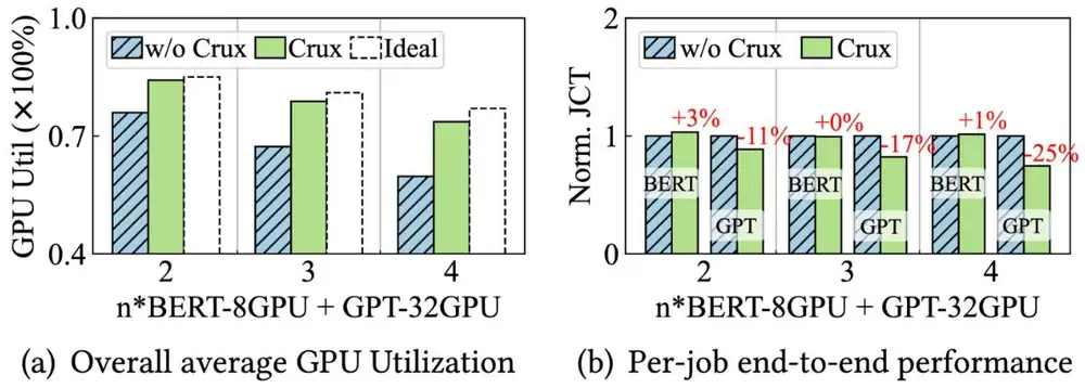
In every row the favored job speeds up a lot and the others lose almost nothing, because their transfers fit into its compute phases (Diagram C).

每一列中，受優待的任務都快了很多，其他任務幾乎沒有損失，因為它們的傳輸塞進了受優待任務的計算階段（示意圖 C）。

Diagram C. The table's measured JCT changes. Dots are stated values; the Fig. 19 bars span the stated range for 2–4 BERT jobs (the paper's Figure 19 above gives each value).示意圖 C。上表的實測 JCT 變化。點是論文給出的數值；Fig. 19 的長條是 2–4 個 BERT 任務時給出的範圍（各個數值見上方的論文圖 19）。Drawn for this primer from Cao et al., SIGCOMM 2024, §6.2 and Figures 19–22 (96-GPU testbed, measured).

Larger-scale results come from an $\alpha$ – $\beta$ simulation of the trace (no queues, PFC or congestion control), so this page does not report them.

更大規模的結果來自追蹤資料的 $\alpha$ – $\beta$ 模擬（沒有佇列、PFC 或壅塞控制），所以本頁不列出。

6. Limits and open questions6. 限制與未解的問題

The paper's own limits: one overlap pattern, a single reference job, no storage traffic, and a throughput loss for low-priority jobs that it measured only in simulation. A careful reader adds:

論文自己的限制：只有一種重疊模式、單一參考任務、沒有儲存流量，以及低優先權任務的吞吐損失（只在模擬中量過）。細心的讀者還應補上：

Scale. 96 GPUs and 2–5 jobs; the large-scale model has no queues or PFC.規模。96 顆 GPU、2–5 個任務；大規模模型沒有佇列與 PFC。
Priorities and PFC. Each lossless class needs buffer headroom; the paper does not say how many of the 8 levels are lossless.優先權與 PFC。每個無損類別都需要緩衝 headroom；論文沒有說 8 個等級中有幾個是無損的。
Starvation. Strict priority can starve a job; the paper relies on bursty traffic. LEVELLER tests this.飢餓。嚴格優先權可能讓任務飢餓；論文依賴流量的突發性。LEVELLER 檢驗了這點。
Text errors. The NIC speed, and §6.2 citing Figures 19–20 for PCIe results (in 21–22).文字錯誤。NIC 速度，以及 §6.2 把 PCIe 結果標成 Figures 19–20（實際在 21–22）。

7. How it connects7. 與其他內容的關聯

LEVELLER (next digest) uses the same knobs (strict priority, few levels, one bottleneck link, graph-based compression, this trace) for the opposite goal: fairness instead of utilization.LEVELLER（下一篇導讀）用同樣的旋鈕（嚴格優先權、少數等級、單一瓶頸鏈路、以圖為基礎的壓縮、這份追蹤資料）追求相反的目標：公平而不是使用率。
Deep dive §2 and its Panel 2 treat placement; Crux keeps placement fixed and schedules the contention that remains. §4's two-line model makes Example 2's point: hidden communication costs nothing.第 11.2 節與其面板 2談配置；Crux 固定配置，排程剩下的競爭。第 4 節的兩行模型與 Example 2 講同一件事：被隱藏的通訊沒有代價。
Guided readings: Alibaba HPN (same team) removes hash collisions by structure, and Crux schedules the rest; DCQCN and Microsoft RoCE explain the priority classes and PFC pauses under Crux's levels.論文導讀：Alibaba HPN（同一團隊）以結構消除雜湊碰撞，Crux 排程其餘部分；DCQCN 與 Microsoft RoCE 解釋了 Crux 等級底下的優先權類別與 PFC 暫停。

Key numbers關鍵數字

Number	數字	Meaning and setup
36.3% / 51%	Jobs / GPUs exposed to contention (production trace)	曝露於競爭的任務 / GPU（生產追蹤）
1.53 → 1.70 s; −9.5%	GPT iteration next to BERT; GPU utilization (measured re-run)	與 BERT 並存時 GPT 的迭代；GPU 使用率（實測重跑）
+8.3–14.8%	GPU utilization gain, 96-GPU testbed	GPU 使用率增益，96 顆 GPU 測試平台
−7 to −33% / +0 to +3%−7 至 −33% / +0 至 +3%	JCT of favored / other jobs, same testbed	受優待 / 其他任務的 JCT，同一測試平台

Terms used on this page本頁用到的術語

GPU intensity: $I_j = W_j / t_j$ : computation per iteration over communication time on the bottleneck link.; $I_j = W_j / t_j$ ：每次迭代的計算量除以瓶頸鏈路上的通訊時間。
Correction factor $k_j$: Multiplier on intensity for iteration length and overlap, found against a reference job.; 為迭代長度與重疊而乘在強度上的倍數，與參考任務比較求得。
Contention DAG: Jobs as nodes; an edge from the higher- to the lower-priority job of each pair sharing a link.; 以任務為節點；共用鏈路的每對任務，從優先權較高者連邊到較低者。