Research digest 5 of 5 · Chapter 11: Sharing the cluster

研究導讀 5 / 5 · 第 11 章：共用叢集

Supercharging Packet-level Network Simulation of Large Model Training via Memoization and Fast-Forwarding以記憶化與快轉大幅加速大型模型訓練的封包級網路模擬

NSDI 2026Fei Long, Kaihui Gao, Li Chen et al. (Tsinghua University, Zhongguancun Laboratory, Huawei) · paper論文

After reading, you can explain how Wormhole skips over 99.5% of ns-3's packet events yet stays packet-level: memoize repeated contention, fast-forward steady rates, and count speedup in events.讀完後，你能說明 Wormhole 如何略過 ns-3 超過 99.5% 的封包事件，卻仍維持封包級：記住重複的競爭、快轉穩定的速率，並以事件數計算加速。

≈ 11 min · 1 interactive panel · 5-question quiz≈ 11 分鐘 · 1 個互動面板 · 5 題測驗Chapter 11 ↗第 11 章 ↗Jump to the quiz ↓跳到測驗 ↓

If you read nothing else

只讀這一段也可以

Packet-level simulators such as ns-3 show queues, PFC and congestion control at work, and training simulators such as SimAI use them. They are slow: a GPT-13B workload on 128 GPUs took 9 hours to simulate, and one GPT-3 175B iteration takes weeks. Wormhole removes events instead of coarsening the model. Training traffic repeats: a real 256-GPU trace holds 65,870 contention instances but only 1,488 distinct patterns, and flows spend most of their time at a steady rate. Wormhole replays a convergence from memory when its flow conflict graph recurs, and skips steady periods. On a 56-core server the paper reports 227–745× speedup over ns-3 on GPT workloads, a peak of 1,012× with Unison across network sizes, and more than 99.5% of events skipped. Against a real trace its end-to-end error was 3.02%.

ns-3 這類封包級模擬器能呈現佇列、PFC 與壅塞控制的實際運作，SimAI 等訓練模擬器也採用它。但它很慢：128 顆 GPU 上的 GPT-13B 工作負載要模擬 9 小時，GPT-3 175B 的一次迭代要好幾週。Wormhole 去除事件，而不是把模型變粗。訓練流量會重複：一份真實的 256 顆 GPU 軌跡有 65,870 個競爭實例，卻只有 1,488 種不同的模式，而且流大部分時間都處在穩定速率。流衝突圖再次出現時，Wormhole 從記憶中重播收斂過程，並略過穩定期。在 56 核心的伺服器上，論文報告在 GPT 工作負載上比 ns-3 加速 227–745 倍，搭配 Unison 在各網路規模中的峰值為 1,012 倍，並略過超過 99.5% 的事件。對照真實軌跡，端到端誤差為 3.02%。

1. Where this paper sits1. 這篇論文的位置

Section 12.2 ("What a simulator adds") says a flow-level simulator is fast enough for 10,000 GPUs, while a far slower packet-level one is the only level that reproduces hash polarization or a victim flow. SimAI keeps ns-3 and pays in run time. Before Wormhole there were two ways out. Flow-level and learned models are fast, but their flow completion times (FCT) differ from ns-3 by about 20% and 10–15%. Parallel simulators such as Unison and DONS keep fidelity, but threads must synchronize, and Unison stayed below 10×.

第 12.2 節（「模擬器多了什麼」）說，流級模擬器快到足以處理 10,000 顆 GPU，而慢得多的封包級模擬器是唯一能重現 hash polarization 或受害者流的層級。SimAI 保留 ns-3，付出的是執行時間。在 Wormhole 之前有兩條出路。流級與學習式模型很快，但它們的流完成時間（FCT）與 ns-3 相差約 20% 與 10–15%。Unison 與 DONS 這類平行模擬器保有保真度，但執行緒必須同步，Unison 停在 10 倍以下。

2. The problem, measured2. 問題，用量測說話

The paper reports the cost on a 56-core server (Figure 2 of the paper). ns-3's run time grows steeply with cluster size and reaches weeks for one GPT-3 175B iteration, and a GPT-13B workload on 128 GPUs took 9 hours. A training run produces more than $10^{12}$ packet events. Two observations make a shortcut possible (Figure 1).

論文報告了在 56 核心伺服器上的代價（論文 Figure 2）。ns-3 的執行時間隨叢集規模急遽增加，GPT-3 175B 的一次迭代要好幾週，128 顆 GPU 上的 GPT-13B 工作負載要 9 小時。一次訓練會產生超過 $10^{12}$ 個封包事件。兩項觀察讓捷徑成為可能（圖 1）。

Figure 1. The motivation of §1–§2, redrawn. ① and ③–④ are the paper's measurements, while ② follows the shape of the paper's Figure 2b and its stated ceiling.圖 1。重畫 §1–§2 的動機。① 與 ③–④ 是論文的量測，② 則依論文 Figure 2b 的形狀與它說明的上限繪製。Drawn for this primer from Long et al., NSDI 2026, §1, §2.1–§2.3 and §7.1.

A contention pattern is a set of flows that overlap, plus the links they share. In a real trace of GPT-18B training on 256 A100 GPUs, the authors count 65,870 contention instances but only 1,488 distinct patterns, because the same collectives run again and again. In the same trace, flows spend 98.82% of their time in a steady state, where congestion control has converged and the rate stays flat. The paper does not say whether these come straight from the trace or from a replay of it; its SimAI-generated counts are simulated and not repeated here.

競爭模式（contention pattern）是一組彼此重疊的流，加上它們共用的鏈路。在一份 256 顆 A100 GPU 訓練 GPT-18B 的真實軌跡中，作者數到 65,870 個競爭實例，卻只有 1,488 種不同的模式，因為同樣的集體操作一再執行。在同一份軌跡中，流有 98.82% 的時間處在穩定狀態：壅塞控制已經收斂，速率保持平坦。論文沒有說明這些數字是直接取自軌跡，還是來自軌跡的重播；它用 SimAI 產生的數字是模擬的，這裡不重複。

3. The design3. 設計

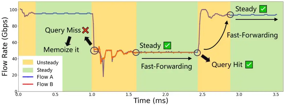
Wormhole is a kernel inside ns-3, not a new model: every packet it simulates is an ns-3 packet. It wraps the event loop in seven steps (§3.2); the paper's Figure 1, after the list, shows the main ones on two flows:

Wormhole 是 ns-3 內部的核心，不是新的模型：它模擬的每個封包都是 ns-3 的封包。它用七個步驟包住事件迴圈（§3.2）；清單後的論文 Figure 1 在兩條流上示範其中主要的步驟：

Split the network into port-level partitions.把網路切成埠級分區。
Look up each new partition in a database.到資料庫查詢每個新分區。
Hit: jump to the stored end of convergence; miss: simulate packets.命中時跳到儲存的收斂終點；未命中時模擬封包。
Watch each flow's rate for a steady state.觀察每條流的速率是否進入穩定狀態。
Fast-forward a steady partition to its next event.把穩定的分區快轉到下一個事件。
Store each newly simulated convergence.儲存每次新模擬的收斂過程。
Re-partition when a flow starts or ends.有流開始或結束時重新分區。

Flow rate versus time for two flows with alternating unsteady and steady regions, annotated with query miss, memoize, fast-forwarding and query hit — The paper's Figure 1, an illustration on two simulated flow rates. Steady periods (green) are fast-forwarded; an unsteady period (yellow) is simulated and memoized on a miss, and skipped on a later hit.論文的 Figure 1，畫在兩條模擬流速率上的示意圖。穩定期（綠色）被快轉；不穩定期（黃色）在未命中時被模擬並記住，之後命中時就略過。Screenshot of Long et al., NSDI 2026 (USENIX PDF).

3.1 Memoization: partitions and the flow conflict graph3.1 記憶化：分區與流衝突圖

A partition is a set of flows that share a port or link, with the links they cross; partitions share no links (Definition 1). Wormhole builds a bipartite graph of flows and links and finds its connected components by depth-first search in $O(N+M)$ time for $N$ flows and $M$ links, and it updates them incrementally as flows come and go. It cuts at ports rather than switches because ports on one switch barely interfere. Smaller partitions repeat more often, run in parallel, and reach steady state more often.

分區是一組共用某個埠或鏈路的流，連同它們經過的鏈路；分區之間不共用鏈路（Definition 1）。Wormhole 建立流與鏈路的二分圖，用深度優先搜尋找出連通分量，對 $N$ 條流與 $M$ 條鏈路只需 $O(N+M)$ 時間，並在流加入或離開時增量更新。它在埠而不是交換器上切分，因為同一台交換器的各個埠幾乎互不干擾。分區越小，越常重複、越能平行執行，也越常進入穩定狀態。

Figure 2. Memoization (§4). f1 and f2 share three links and form P1; f3 uses other ports of leaf B and forms P2. Later, f7 and f9 form the same weighted graph, so their convergence is skipped.圖 2。記憶化，依論文 §4 繪製。f1 與 f2 共用三條鏈路，構成 P1；f3 使用 leaf B 的其他埠，構成 P2。之後 f7 與 f9 構成加權形狀相同的圖，所以它們的收斂過程被略過。Drawn for this primer from Long et al., NSDI 2026, §4.1–§4.4.

Each partition is summarized by a flow conflict graph (FCG): one vertex per flow, weighted by its current rate, and an edge between two flows that share links, weighted by the number of shared links (Figure 2). The key is the FCG when the partition forms; the value is the FCG when convergence ends, each flow's bytes sent during it, and the convergence time $T_{\text{conv}}$ . A lookup filters by vertex and edge counts, then tests weighted graph isomorphism. On a hit, Wormhole skips the convergence and applies the stored bytes and time. At 1,024 GPUs the database stays under 100 KB.

每個分區由一張流衝突圖（flow conflict graph，FCG）概括：每條流一個頂點，權重是它當下的速率；共用鏈路的兩條流之間有一條邊，權重是共用鏈路的數量（圖 2）。鍵是分區形成時的 FCG；值是收斂結束時的 FCG、每條流在收斂期間送出的位元組，以及收斂時間 $T_{\text{conv}}$ 。查詢時先依頂點與邊的數量過濾，再測試加權圖同構。命中時，Wormhole 略過收斂過程，套用儲存的位元組與時間。在 1,024 顆 GPU 時，資料庫小於 100 KB。

3.2 Fast-forwarding steady states3.2 快轉穩定狀態

Wormhole watches one quantity per flow, the sending rate $R$ . Over the last $l$ rate samples it computes the relative spread

Wormhole 對每條流只觀察一個量：傳送速率 $R$ 。它對最近 $l$ 個速率樣本計算相對變動幅度

\Delta R_l = \frac{\max_{k} R(t_k) - \min_{k} R(t_k)}{\frac{1}{l}\sum_{k=1}^{l} R(t_k)}

and calls the flow steady when $\Delta R_l < \theta$ , with $\theta = 5\%$ and $l = 2{,}000$ by default. The steady rate $\hat R$ is the window's mean, not a max-min fair share, which converged congestion control need not reach. A partition is steady when all its flows are. Theorem 1 shows why one quantity is enough: through $\mathit{cwnd} = R \times \mathrm{RTT}$ and TIMELY and DCTCP models, a small spread in $R$ bounds the window, RTT, queue and bytes in flight. Theorems 2 and 3 bound the error of a skip:

當 $\Delta R_l < \theta$ 時就判定這條流穩定，預設 $\theta = 5\%$ 、 $l = 2{,}000$ 。穩定速率 $\hat R$ 取視窗內的平均，而不是收斂後的壅塞控制未必會達到的 max-min 公平分配。分區內所有流都穩定時，分區才算穩定。Theorem 1 說明為何一個量就夠：透過 $\mathit{cwnd} = R \times \mathrm{RTT}$ 以及 TIMELY 與 DCTCP 的模型， $R$ 的小幅變動限制了視窗、RTT、佇列與在途位元組。Theorem 2 與 3 給出略過的誤差上限：

\frac{|\hat R - R|}{R} < \frac{\theta}{1-\theta}, \qquad \frac{|\hat T - T|}{T} < \theta

At $\theta = 5\%$ the rate bound is about 5.3%. A steady partition then skips to its next interrupt: a known flow arrival, a computed completion, or a reroute. If an unplanned event arrives before that point, Wormhole skips back to it (Figure 3).

在 $\theta = 5\%$ 時，速率誤差上限約 5.3%。穩定的分區接著跳到下一個中斷：已知的流到達、算出的完成時刻，或改道。若有未預期的事件在那之前到來，Wormhole 就倒回到該事件（圖 3）。

Figure 3. Fast-forwarding one flow, with a rate trace drawn after §5. After

l

samples within

\theta

of their mean, the rest of the steady phase is skipped, and when a new flow joins, its pattern hits the database and the convergence is replayed.圖 3。快轉一條流，速率軌跡依論文 §5 繪製。一旦

l

個樣本都落在平均的

\theta

範圍內，穩定期的其餘部分就被略過。新流加入時，新的模式在資料庫中命中，所以它的收斂過程是重播的。Drawn for this primer from Long et al., NSDI 2026, §3.2 and §5.1–§5.3.

Skipping changes how speed should be counted. Appendix I defines the speedup $S$ as "the quotient of events processed by ns-3 divided by events processed by Wormhole." If a fraction $f$ of the events is skipped,

略過事件改變了速度該怎麼算。附錄 I 把加速 $S$ 定義為「ns-3 處理的事件數除以 Wormhole 處理的事件數」。若有比例 $f$ 的事件被略過，

S = \frac{E_{\text{ns-3}}}{E_{\text{Wormhole}}} = \frac{1}{1-f}

so the measured $f > 99.5\%$ on GPT workloads means $S > 200$ . Near the top, each extra tenth of a percent matters: $f = 99.9\%$ gives $S = 1{,}000$ . The panel builds $f$ from a periodic training step.

所以 GPT 工作負載上實測的 $f > 99.5\%$ 代表 $S > 200$ 。在接近頂端時，每多千分之一都很重要： $f = 99.9\%$ 就得到 $S = 1{,}000$ 。下面的面板用週期性的訓練步來組出 $f$ 。

Panel 1面板 1

Fast-forward and memoize one training step, counted in events對一個訓練步做快轉與記憶化，以事件數計算

Steady length

L

(× convergence)穩定期長度

L

（收斂期倍數）

Repeats

R

of a pattern per step同一模式每步重複

R

次

Fast-forward steady states快轉穩定狀態

Memoize convergence記憶收斂過程

Events simulated / ns-3

模擬的事件 / ns-3

Events skipped

略過的事件

Event-count speedup

事件數加速

Fast-forward alone · memo factor

單靠快轉 · 記憶化倍數

Our model, not the paper's simulator. One contention pattern recurs $R$ times per training step. Each instance converges for one time unit, then holds a steady rate for $L$ units, and every unit costs the same number of packet events, so ns-3 simulates $R(1+L)$ units. Fast-forwarding skips each steady phase; memoization replays every convergence after the first. Speedup is counted in events, as Appendix I defines it. Defaults come from the real GPT-18B trace: 98.82% of flow time steady ( $L = 84$ ) and 65,870 instances of 1,488 patterns ( $R \approx 44$ ). The model is an upper bound: it detects steady states at once and lets every repeat hit the database. Measured on GPT workloads: fast-forwarding alone gave more than 130× and memoization a further 1.93–8.43× (Fig. 9a); each flow entered steady state about 0.94 times on average; the real trace ran 97.75× faster (Fig. 14).

這是我們的模型，不是論文的模擬器。同一個競爭模式每個訓練步重複 $R$ 次。每個實例先收斂一個時間單位，再以穩定速率維持 $L$ 個單位，而每個單位耗費相同數量的封包事件，所以 ns-3 要模擬 $R(1+L)$ 個單位。快轉略過每段穩定期；記憶化重播第一次之後的每次收斂。加速以事件數計算，與附錄 I 的定義相同。預設值來自真實的 GPT-18B 軌跡：98.82% 的流時間處於穩定（ $L = 84$ ），1,488 種模式共 65,870 個實例（ $R \approx 44$ ）。這個模型是上限：它立刻偵測到穩定狀態，並讓每次重複都在資料庫中命中。GPT 工作負載的實測：單靠快轉超過 130 倍，記憶化再乘上 1.93–8.43 倍（Fig. 9a）；每條流平均約進入穩定狀態 0.94 次；真實軌跡快了 97.75 倍（Fig. 14）。

Stop and think停下來想一想

Set $L = 129$ and turn memoization off: the model gives 130×, the paper's measured floor for fast-forwarding alone. Now turn memoization on. The model multiplies by $R$ ; the paper measured 1.93–8.43×. Which assumptions of the model break in real traffic?

把 $L$ 設為 129 並關掉記憶化：模型給出 130 倍，正是論文單靠快轉的實測下限。現在打開記憶化。模型乘上 $R$ ；論文實測只有 1.93–8.43 倍。模型的哪些假設在真實流量中不成立？

4. Implementation4. 實作

Wormhole adds thousands of lines to ns-3.17 (the HPCC version) and Open-USim (Huawei's ns-3-ub). Three details keep a skip consistent. Packet pausing: the ports of a steady partition stop processing packets but keep their buffer occupancy, so other partitions see the same free buffer. Timestamp offset: the global clock keeps running, and a partition that skips by $T$ adds $T$ to its pending events and advances its flow sizes and sequence numbers. Unison integration: the port-level partitions become Unison's logical processes, database lookups run in parallel, and inserts take fine-grained locks.

Wormhole 在 ns-3.17（HPCC 版）與 Open-USim（華為的 ns-3-ub）上增加了數千行程式碼。三個細節讓略過保持一致。暫停封包：穩定分區的埠停止處理封包，但保留緩衝區占用量，讓其他分區看到相同的可用緩衝。時間戳位移：全域時鐘繼續走，略過 $T$ 的分區把待處理事件加上 $T$ ，並推進流的大小與序號。與 Unison 整合：埠級分區成為 Unison 的邏輯處理單元，資料庫查詢平行執行，寫入則用細粒度鎖。

5. What was measured5. 量到了什麼

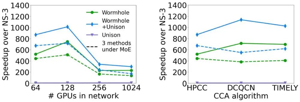
The server has two Intel Xeon CPUs (56 cores) and 128 GB of memory. The fabrics are rail-optimized fat-trees of 64, 128, 256 and 1,024 GPUs, each GPU a host. GPT and MoE workloads carry DP, PP and EP flows with micro-batch 1; TP and SP stay on NVLink and are left out. HPCC is the default congestion control, with DCQCN and TIMELY as variants. Baselines are ns-3, Unison and a flow-level simulator. Wormhole alone ran on one core; Wormhole+Unison used 16.

伺服器有兩顆 Intel Xeon CPU（56 核心）與 128 GB 記憶體。網路是 64、128、256 與 1,024 顆 GPU 的 rail-optimized fat-tree，每顆 GPU 視為一台主機。GPT 與 MoE 工作負載承載 DP、PP 與 EP 的流，micro-batch 為 1；TP 與 SP 留在 NVLink 上，不納入。預設壅塞控制是 HPCC，另以 DCQCN 與 TIMELY 為變化。比較基準是 ns-3、Unison 與一個流級模擬器。Wormhole 單獨跑在一個核心上；Wormhole+Unison 用 16 個核心。

Two line charts of speedup over ns-3: versus number of GPUs, and versus congestion control algorithm — The paper's Figure 8: speedup over ns-3 by network size (left, HPCC) and by congestion control (right, 64 GPUs); solid GPT, dashed MoE. Appendix I defines this speedup as an event-count ratio.論文的 Figure 8：相對 ns-3 的加速，左為依網路規模（HPCC），右為依壅塞控制（64 顆 GPU）；實線 GPT，虛線 MoE。附錄 I 把這個加速定義為事件數的比值。Screenshot of Long et al., NSDI 2026 (USENIX PDF).

Two units of speed. Wall-clock time appears only as absolute times: Wormhole+Unison cut a GPT-13B workload on 128 GPUs "from 9 hours to 5 minutes," and ns-3 takes weeks per GPT-3 175B iteration. The paper defines "speedup" only in Appendix I, as a ratio of event counts; the skipped-event shares are event counts too. How the +Unison figures fit that definition is unclear, since Unison runs events in parallel rather than removing them.

兩種速度單位。牆鐘時間只以絕對時間的形式出現：Wormhole+Unison 把 128 顆 GPU 上的 GPT-13B 工作負載「從 9 小時降到 5 分鐘」，而 ns-3 每次 GPT-3 175B 迭代要好幾週。論文只在附錄 I 定義「加速」，即事件數的比值；略過事件的比例也是事件數。+Unison 的數字如何符合這個定義並不清楚，因為 Unison 是平行執行事件，而不是去除事件。

Result (paper figure)結果（論文圖）	Setup設定	Value數值
Speedup over ns-3 (Fig. 8a)相對 ns-3 的加速（Fig. 8a）	64–1,024 GPUs, HPCC, one core64–1,024 顆 GPU，HPCC，單核心	227–745× GPT · 135–510× MoEGPT 227–745 倍 · MoE 135–510 倍
With Unison (Fig. 8a)搭配 Unison（Fig. 8a）	16 cores, peak across sizes; Unison alone < 10×16 核心，各規模中的峰值；Unison 單獨 < 10 倍	1,012× GPT · 716× MoEGPT 1,012 倍 · MoE 716 倍
Breakdown (Fig. 9a)拆解（Fig. 9a）	fast-forward alone; memoization on top單靠快轉；再加上記憶化	> 130× GPT, > 50× MoE; × 1.93–8.43GPT > 130 倍、MoE > 50 倍；× 1.93–8.43
Events skipped (Fig. 9b)略過的事件（Fig. 9b）	event count事件數	> 99.5% GPT · > 99.2% MoEGPT > 99.5% · MoE > 99.2%
FCT error (Fig. 10a)FCT 誤差（Fig. 10a）	against ns-3, not hardware對照 ns-3，不是硬體	within 1% (flow-level ≈ 20%)1% 以內（流級約 20%）
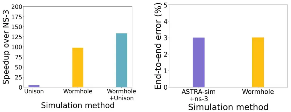
Real trace (Fig. 14)真實軌跡（Fig. 14）	GPT-18B, 256 GPUs, TP8-DP16-PP2-VPP2; Nsight Compute ground truthGPT-18B，256 顆 GPU，TP8-DP16-PP2-VPP2；以 Nsight Compute 為基準真值	3.02% error (ASTRA-sim + ns-3: 3.01%); 97.75× · 133.35× with Unison誤差 3.02%（ASTRA-sim + ns-3：3.01%）；97.75 倍 · 搭配 Unison 133.35 倍

Figure 4. The reported speedups on one log axis. The green line marks 200×, which

f = 99.5\%

implies. Synthetic workloads sit to its right, the real trace to its left. Synthetic accuracy is against ns-3; the trace row is against measured training time.圖 4。論文報告的加速，畫在同一條對數軸上。綠線標出

f = 99.5\%

所對應的 200 倍。合成工作負載在它右邊，真實軌跡在它左邊。合成工作負載的精確度是對照 ns-3；軌跡那一列則是對照實測的訓練時間。Drawn for this primer from Long et al., NSDI 2026, §7.1–§7.4, Figures 8, 9, 10 and 14.

Three readings matter. First, the 1% FCT error is fidelity to ns-3, a simulator. The only hardware comparison is the real trace, where Wormhole was within 3.02%, as close as ASTRA-sim with plain ns-3 (3.01%). Second, on that trace the speedup was 97.75×, well below the synthetic 227–745×.

有三個重點。第一，1% 的 FCT 誤差是對 ns-3 這個模擬器的保真度。唯一與硬體的比較是真實軌跡：Wormhole 的誤差在 3.02% 以內，與 ASTRA-sim 搭配原版 ns-3 的 3.01% 一樣接近。第二，在那份軌跡上加速是 97.75 倍，遠低於合成工作負載的 227–745 倍。

Two bar charts: speedup over ns-3 for three methods, and end-to-end error for ASTRA-sim plus ns-3 and Wormhole — The paper's Figure 14, the real 256-GPU trace. Left: speedup over ns-3. Right: error against measured training time, 3.01% for ASTRA-sim + ns-3 and 3.02% for Wormhole.論文的 Figure 14，真實的 256 顆 GPU 軌跡。左：相對 ns-3 的加速。右：相對實測訓練時間的誤差，ASTRA-sim + ns-3 為 3.01%，Wormhole 為 3.02%。Screenshot of Long et al., NSDI 2026 (USENIX PDF).

Third, memoization added far less than the repetition counts suggest: each flow entered steady state only about 0.94 times on average, and the PP-heavy middle of an iteration gains less (Appendix I). Detection on rate, in-flight bytes or queue length gave similar results, and speed varied by at most 13% across topologies.

第三，記憶化增加的倍數遠小於重複次數所暗示的：每條流平均只進入穩定狀態約 0.94 次，而一次迭代中以 PP 為主的中段加速較少（附錄 I）。以速率、在途位元組或佇列長度偵測，結果相近；在不同拓樸間，速度差異最多 13%。

6. Limits and open questions6. 限制與未解的問題

The paper names three limits. Multi-tenant cloud traffic repeats less and reaches steady state less often; in the worst case Wormhole falls back to ns-3 speed with no added error. Incremental partitioning can degrade to full recomputation. Memoization adds slightly more error than fast-forwarding alone. A careful reader adds:

論文列出三項限制。多租戶雲端流量重複較少、進入穩定狀態也較少；最壞情況下，Wormhole 退回 ns-3 的速度，但不增加誤差。增量分區可能退化成完整重算。記憶化帶來的誤差比單靠快轉稍多。細心的讀者還會補上：

Units. The speedup metric is an event-count ratio by definition; the 9-hour-to-5-minute pair is the only wall-clock evidence for the combined system.單位。加速指標依定義是事件數的比值；「9 小時到 5 分鐘」這一對是合併系統唯一的牆鐘證據。
Workloads. No TP or SP traffic, micro-batch 1, and no failures, stragglers or background tenants, the conditions the sharing papers study.工作負載。沒有 TP 或 SP 流量、micro-batch 為 1，也沒有故障、straggler 或背景租戶，而這正是共享類論文研究的條件。
Untested dynamics. PFC storms, adaptive routing and packet spraying are not evaluated; on-off pauses could confuse a rate test.未測試的動態。PFC 風暴、adaptive routing 與 packet spraying 都沒有評估；時開時停的暫停可能混淆速率測試。
Graph abstraction. The FCG ignores path length, so two isomorphic patterns with different RTTs reuse one convergence time.圖的抽象。FCG 忽略路徑長度，所以兩個 RTT 不同但同構的模式會重用同一個收斂時間。

7. How it connects7. 與其他內容的關聯

Chapter 11, section 4: packet-level runs move toward the scale where only flow-level models fit, paying packet cost only for new traffic.第 11 章第 4 節：封包級模擬往只有流級模型才跑得動的規模推進，只為新的流量付出封包級代價。
SimAI (two shared authors) runs ns-3 with UNISON; Wormhole composes with Unison and took its motivating workloads from SimAI.SimAI（有兩位共同作者）執行搭配 UNISON 的 ns-3；Wormhole 可與 Unison 合用，動機工作負載也取自 SimAI。
Chapter 7 and the DCQCN guided reading: memoization replays the convergence of DCQCN, HPCC or TIMELY.第 7 章與 DCQCN 導讀：記憶化重播的是 DCQCN、HPCC 或 TIMELY 的收斂過程。
Crux, LEVELLER and MonkeyTree evaluate at scale with $\alpha$ – $\beta$ or flow-level models. Wormhole could replace them with packet-level runs, but its gains shrink under multi-tenant traffic, their setting.Crux、LEVELLER 與 MonkeyTree 用 $\alpha$ – $\beta$ 或流級模型做大規模評估。Wormhole 可以用封包級模擬取代它們，但它的增益在多租戶流量下會縮小，而那正是它們的情境。

Key numbers關鍵數字

Number	數字	Meaning (setup)
9 h → 5 min	GPT-13B on 128 GPUs: ns-3 vs Wormhole+Unison (wall clock)	128 顆 GPU 上的 GPT-13B：ns-3 對 Wormhole+Unison（牆鐘時間）
65,870 → 1,488	Contention instances → distinct patterns, real 256-GPU trace	競爭實例 → 不同模式，真實 256 顆 GPU 軌跡
98.82%	Share of flow time in steady state, same trace	流時間中處於穩定狀態的比例，同一份軌跡
$\theta = 5\%$ , $l = 2{,}000$	Detector defaults; rate error below about 5.3%	偵測器預設值；速率誤差約 5.3% 以下
227–745× · 1,012×	Speedup over ns-3 on GPT (event-count metric) · peak with Unison across sizes	GPT 上相對 ns-3 的加速（事件數指標）· 搭配 Unison 在各規模中的峰值
> 99.5%	Events skipped on GPT workloads	GPT 工作負載上略過的事件
< 1% · 3.02%	FCT error vs ns-3 · end-to-end error vs a real trace (ASTRA-sim + ns-3: 3.01%)	相對 ns-3 的 FCT 誤差 · 相對真實軌跡的端到端誤差（ASTRA-sim + ns-3：3.01%）

Terms used on this page本頁用到的術語

Contention pattern: A set of overlapping flows plus the links they share.; 一組彼此重疊的流，加上它們共用的鏈路。
Port-level partition: Flows that share ports or links, isolated from all other flows.; 共用埠或鏈路、與其他所有流隔開的一組流。
Flow conflict graph: Flows as rate-weighted vertices, shared-link counts as edge weights; the memoization key.; 以速率為權重的流作頂點、以共用鏈路數為邊權重；記憶化的鍵。
Steady state: A period in which a flow's rate stays within $\theta$ of its mean over $l$ samples.; 流的速率在 $l$ 個樣本內維持在平均的 $\theta$ 範圍內的期間。
Skip-back: Rewinding a fast-forward when an unplanned event arrives before the skip's end.; 未預期事件在略過終點之前到來時，把快轉倒回。