Research digest 13 of 16 · Chapter 4: Collective communication

研究導讀 13 / 16 · 第 4 章：集體通訊

DynamiQ: Accelerating Gradient Synchronization using Compressed Multi-hop All-reduceDynamiQ：以壓縮的多跳 all-reduce 加速梯度同步

SIGCOMM 2026Wenchen Han, Shay Vargaftik, Michael Mitzenmacher, Ran Ben Basat (UCL, VMware Research by Broadcom, Harvard) · paper論文

After reading, you can explain why compression error grows hop by hop in a ring all-reduce, and how DynamiQ's agreed bit widths, re-fitted scales and correlated rounding keep accuracy near BF16.讀完後，你能說明壓縮誤差為何在環形 all-reduce 中逐跳累積，以及 DynamiQ 如何以一致的位元寬度、每跳重新擬合的尺度與相關捨入，讓精度接近 BF16。

≈ 11 min · 1 interactive panel · 5-question quiz≈ 11 分鐘 · 1 個互動面板 · 5 題測驗Chapter 4 ↗第 4 章 ↗Jump to the quiz ↓跳到測驗 ↓

If you read nothing else

只讀這一段也可以

Most gradient compressors were built for a parameter server, where each worker compresses once and the server adds in high precision. In a multi-hop all-reduce (ring, butterfly), each intermediate GPU adds to a partial sum and sends it on, so it must recompress the sum, adding error at every hop, or send more bits. DynamiQ recompresses and controls the error: a small first all-reduce lets every GPU agree on a width (2, 4 or 8 bits) for each block of 256 values within a 5-bit average, and one fused kernel per hop decompresses, adds and recompresses with re-fitted scales, non-uniform levels and correlated rounding. On eight RTX A6000 GPUs in four servers, fine-tuning LLaMA 1B reached 99% of BF16 accuracy 34.5% faster than MXFP8 and 40.8% faster than BF16; final accuracy stayed within 0.1% of BF16.

大多數梯度壓縮器是為參數伺服器設計的：每個 worker 壓縮一次，伺服器以高精度相加。在多跳 all-reduce（環形、butterfly）中，每個中間 GPU 把資料加進部分和再往下送，所以它要嘛重新壓縮這個和，每一跳都增加誤差，要嘛送更多位元。DynamiQ 選擇重新壓縮並控制誤差：先用一次小型 all-reduce，讓每顆 GPU 對每 256 個值一組的寬度（2、4 或 8 位元）取得一致，平均不超過 5 位元；每一跳再由一個融合 kernel 解壓縮、相加、再壓縮，並使用重新擬合的尺度、非均勻量化階與相關捨入。在四台伺服器、八顆 RTX A6000 GPU 上微調 LLaMA 1B，達到 BF16 精度 99% 的時間比 MXFP8 快 34.5%、比 BF16 快 40.8%；最終精度與 BF16 相差不到 0.1%。

1. Where this paper sits1. 這篇論文的位置

Section 4.2 follows the ring: after step $s$ , the chunk a rank has just received holds the contributions of $s + 2$ ranks. Section 2 draws the butterfly, whose circles count 1, 2, 4, 8 inputs summed. Both are multi-hop: a partial sum passes through GPUs that each add to it.

第 4.2 節追蹤環形演算法：第 $s$ 步之後，一個 rank 剛收到的區塊包含 $s + 2$ 個 rank 的貢獻。第 2 節畫出 butterfly，圓圈中的 1、2、4、8 是已加總的輸入數。兩者都是多跳的：部分和經過一顆顆 GPU，每顆都把自己的值加進去。

Section 9.5 covers two ways to send fewer bytes: add in the switch (EPIC), or code without loss (ZipCCL, which avoids additions on the path by summing at the destination). The lossy case on a multi-hop path is new on this site. The paper argues that THC, OmniReduce and the microscaling formats MXFP4/6/8 were not built for it.

第 9.5 節介紹兩種少送位元組的方法：在交換器內相加（EPIC），或無損編碼（ZipCCL，它在目的端加總，避開路徑上的加法）。多跳路徑上的有損情形是本站的新內容。論文認為 THC、OmniReduce 與 MXFP4/6/8 等微縮放格式都不是為此設計的。

2. The problem, measured2. 問題，用量測說話

A parameter server quantizes each worker's gradient once. In a ring the first worker quantizes its chunk; the next decompresses it, adds its own and quantizes the sum of two, and so on (Diagram A). A sum of $m$ workers can be $m$ times larger, and quantization error grows with the square of the range it covers, so later hops add more error.

參數伺服器對每個 worker 的梯度只量化一次。環形中第一個 worker 量化自己的區塊；下一個解壓縮、加上自己的區塊，再量化兩個 worker 的和，依此類推（示意圖 A）。 $m$ 個 worker 的和可能大 $m$ 倍，而量化誤差隨它涵蓋的範圍平方成長，所以越後面的跳增加越多誤差。

Diagram A. Error added while four workers sum one chunk, in units of the error of quantizing one worker's values. A parameter server quantizes each value once (4 units); in a ring, hop

k

quantizes a sum of

k

workers (

k^2

units, 14 in all). Both then send

\Sigma_4

, adding the same 16 units.示意圖 A。四個 worker 加總一個區塊時增加的誤差，以「量化一個 worker 的值」的誤差為單位。參數伺服器每個值只量化一次（4 單位）；環形中第

k

跳量化

k

個 worker 的和（

k^2

單位，共 14）。兩者之後都送出

\Sigma_4

，同樣增加 16 單位。Drawn for this primer from the worst-case analysis in Han et al., SIGCOMM 2026, §1 and Appendix B.

The alternative is to keep sums exact and widen the numbers. THC adds integers, so a sum of 4-bit values from $n$ workers needs $b \ge \lceil \log_2(15n + 1) \rceil$ bits to avoid overflow: the bytes grow with $n$ .

另一條路是讓和保持精確、把數字加寬。THC 做整數加法， $n$ 個 worker 的 4 位元值相加需要 $b \ge \lceil \log_2(15n + 1) \rceil$ 位元才不會溢位：位元組隨 $n$ 增加。

The opportunity comes from a measurement. On the first gradient of fine-tuning LLaMA 1B (MMLU) and Gemma 1B (UltraChat), the $\ell_2$ norms of super-groups of 256 entries showed strong locality compared with a random shuffle: about 20% (LLaMA) and 30% (Gemma) were orders of magnitude below the median. Such blocks need few bits. Per-entry widths would cost too much to send and would break byte alignment, fused kernels and coalesced access.

機會來自一項量測。在微調 LLaMA 1B（MMLU）與 Gemma 1B（UltraChat）的第一個梯度上，與隨機打亂相比，256 個元素一組的超群組的 $\ell_2$ 範數呈現強烈的局部性：約 20%（LLaMA）與 30%（Gemma）比中位數小好幾個數量級。這些區塊只需要很少位元。逐元素決定寬度則傳送成本太高，還會破壞位元組對齊、融合 kernel 與合併存取。

3. The design3. 設計

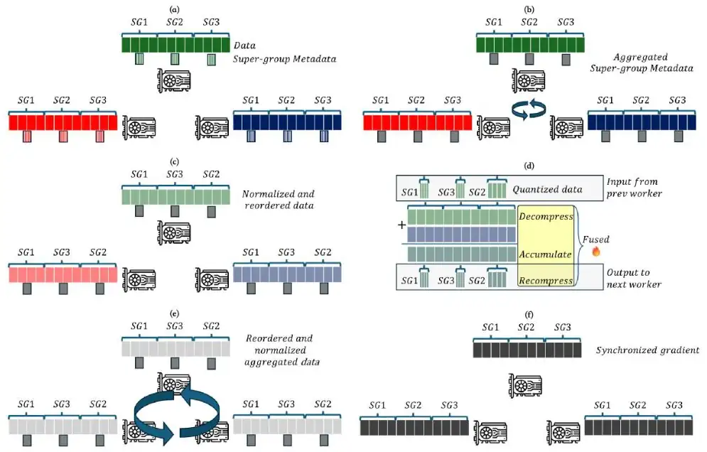
Each training step runs six stages (the paper's Figure 2, below the list, draws them on three workers):

每個訓練步驟執行六個階段（清單下方論文的 Figure 2 以三個 worker 畫出它們）：

Each worker computes the mean and squared norm of each super-group.每個 worker 計算每個超群組的平均值與平方範數。
A lightweight all-reduce sums these statistics.一次輕量 all-reduce 加總這些統計量。
Each worker subtracts the global mean, picks bit widths, and reorders super-groups by width.每個 worker 減去全域平均值、選定位元寬度，並依寬度重排超群組。
The main all-reduce runs with fused kernels.以融合 kernel 執行主要的 all-reduce。
All workers now hold the same sums.所有 worker 得到相同的和。
Each worker adds the means back and restores the order.每個 worker 把平均值加回，並還原順序。

Six panels showing gradient vectors split into super-groups SG1 to SG3 across three GPUs, with metadata exchange, reordering, a fused decompress-accumulate-recompress kernel, all-gather and restore. — Figure 2 of the paper: the DynamiQ workflow (a design diagram, panels (a)–(f)). The key step is (d): every hop decompresses, adds and recompresses inside one fused kernel, using bit widths that all workers agreed on in (b), so the error stays bounded as partial sums grow.論文圖 2：DynamiQ 的流程（設計示意圖，(a) 到 (f)）。關鍵在 (d)：每一跳都在同一個融合 kernel 內解壓縮、相加、再壓縮，使用的位元寬度是所有 worker 在 (b) 中事先同意的，所以部分和變大時誤差仍有上限。Han, Vargaftik, Mitzenmacher and Ben Basat, SIGCOMM 2026, Figure 2 (arXiv 2602.08923 HTML; panels re-arranged 2 × 3).

3.1 Agree on the bit widths first3.1 先對位元寬度取得一致

Worker $i$ computes, for super-group $j$ , the mean $\mu_{i,j}$ and the squared norm $F_{i,j}$ , and the lightweight all-reduce combines them:

worker $i$ 為超群組 $j$ 計算平均值 $\mu_{i,j}$ 與平方範數 $F_{i,j}$ ，輕量 all-reduce 把它們合併：

\mu_j = \frac{1}{n}\sum_{i=1}^{n} \mu_{i,j}, \qquad F_j = \sum_{i=1}^{n} F_{i,j}, \qquad F_{i,j} = \sum_{x \in X_{i,j}} x^2

Each worker subtracts $\mu_j$ and maps $F_j$ to a width: 2 bits below $T_{2,4}$ , 4 bits below $T_{4,8}$ , else 8 (16, uncompressed, is also possible). All workers see the same $F_j$ , so all workers and hops use the same widths and the layout never changes along the path.

每個 worker 減去 $\mu_j$ ，並把 $F_j$ 對應到寬度：低於 $T_{2,4}$ 用 2 位元，低於 $T_{4,8}$ 用 4 位元，否則用 8 位元（也可用不壓縮的 16 位元）。所有 worker 看到相同的 $F_j$ ，所以所有 worker 與每一跳都用相同寬度，資料配置沿路不變。

The thresholds follow one rule: each extra bit halves the quantization step and cuts the worst-case error about 4×. Moving a super-group from $a$ to $b$ bits saves error in proportion to $T_{a,b}(4^{-a} - 4^{-b})$ for $b - a$ bits per entry. Equal saving per bit at every threshold gives

門檻遵循一條規則：每多一個位元，量化間距減半，最壞情況的誤差約降為四分之一。把一個超群組從 $a$ 位元升到 $b$ 位元，以每元素 $b - a$ 位元換得正比於 $T_{a,b}(4^{-a} - 4^{-b})$ 的誤差減少。令每個門檻上每位元的節省相等，得到

\tfrac{3}{16}\,T_{1,2} = \tfrac{15}{512}\,T_{2,4} = \tfrac{255}{4^{9}}\,T_{4,8} \quad\Rightarrow\quad T_{1,2} = \tfrac{5}{32}\,T_{2,4}, \qquad T_{2,4} = \tfrac{17}{512}\,T_{4,8}

One free parameter remains: Appendix A sets each width from $\log_2 F_j$ plus an offset $u$ , without sorting, and tunes $u$ across rounds until the bits fit the budget $\bar b$ , which counts the metadata too:

還剩一個自由參數：附錄 A 由 $\log_2 F_j$ 加上偏移 $u$ 決定每個寬度，不必排序，並在各回合間調整 $u$ ，直到位元數符合預算 $\bar b$ ；預算也包含中繼資料：

Question問題	Calculation算式	Result結果
Lightweight all-reduce: two BF16 numbers per 256 values輕量 all-reduce：每 256 個值兩個 BF16 數	$32 \div 256$	$0.125$ bits位元
Group scale: one UINT8 per 16 values群組尺度：每 16 個值一個 UINT8	$8 \div 16$	$0.5$ bits位元
Super-group scale: one BF16 per 256 values超群組尺度：每 256 個值一個 BF16	$16 \div 256$	$0.0625$ bits位元
Left for the values, at $\bar b = 5$ 留給量化值的位元， $\bar b = 5$ 時	$5 - 0.125 - 0.5 - 0.0625$	$4.3125$ bits位元split among 2-, 4-, 8-bit super-groups分給 2、4、8 位元的超群組
Bits each worker sends per coordinate, ring of 44 個 worker 的環中，每個 worker 每座標送出的位元	$2 \times \tfrac{3}{4} \times 5$	$7.5$ bits位元BF16: 24BF16：24

Finally, each worker sorts super-groups by width, locally and without communication, so each fused kernel sees long runs of one width (Diagram B).

最後，每個 worker 在本地、不經通訊地依寬度排序超群組，讓每個融合 kernel 處理的都是同一寬度的長段資料（示意圖 B）。

Diagram B. Top: where the 5-bit budget goes with the default sizes. Bottom: the agreed energy

F_j

of a super-group picks its width; the two thresholds keep the ratio 512/17, and one offset moves both until the average fits.示意圖 B。上：預設大小下 5 位元預算的去向。下：超群組一致的能量

F_j

決定它的寬度；兩條門檻維持 512/17 的比例，由一個偏移量同時移動，直到平均值符合預算。Drawn for this primer from Han et al., SIGCOMM 2026, §3.2, §3.5 and Appendix A.

3.2 Make each re-quantization cheaper3.2 讓每次重新量化的代價更小

Within a group, entries are divided by the group's largest magnitude and rounded to one of $2^{b-1}$ levels plus a sign bit. Stochastic rounding picks the upper level with probability proportional to the distance from the lower one, so the estimate is unbiased. The levels are not uniform:

在群組內，元素先除以群組的最大絕對值，再捨入到 $2^{b-1}$ 個量化階之一，另加一個符號位元。隨機捨入以「與下鄰階的距離」成正比的機率選上鄰階，所以估計是無偏的。量化階並不均勻：

f(\epsilon, r) = \frac{(1+2\epsilon^2)^{r} - 1}{(1+2\epsilon^2)^{2^{b-1}-1} - 1}, \qquad r = 0, \dots, 2^{b-1}-1

A larger $\epsilon$ puts more levels near zero, where most entries are; the paper does not state its value.

$\epsilon$ 越大，越多量化階集中在大多數元素所在的零附近；論文沒有說明它採用的值。

Hierarchical scales. The super-group's largest magnitude travels in BF16, and each group scale is a stochastically rounded UINT8 fraction of it, $sf_G = r_G \cdot sf_{\mathcal{G}}/255$ . The two roundings are independent, so $\mathbb{E}[\hat x] = \mathbb{E}[\hat{x}']\,\mathbb{E}[sf_G] = x$ : still unbiased.

階層式尺度。超群組的最大絕對值以 BF16 傳送，每個群組尺度則是它的一個經隨機捨入的 UINT8 分數， $sf_G = r_G \cdot sf_{\mathcal{G}}/255$ 。兩次捨入彼此獨立，所以 $\mathbb{E}[\hat x] = \mathbb{E}[\hat{x}']\,\mathbb{E}[sf_G] = x$ ：仍然無偏。

Correlated rounding. A worker rounds up when a uniform draw $u_i$ falls below its rounding probability. DynamiQ uses $u_i = (\pi_i + \gamma_i)/n$ , where $\pi$ is a permutation of $0, \dots, n-1$ from a shared seed (never sent) and $\gamma_i$ is uniform on $[0, 1)$ . Each $u_i$ stays uniform, so rounding stays unbiased, but exactly one $u_i$ falls in each interval of width $1/n$ , so ups and downs pair off (Diagram C). For two workers holding $x = \tfrac12$ , the variance of the 1-bit sum drops from $\tfrac12$ to 0.

相關捨入。worker 在均勻亂數 $u_i$ 小於其進位機率時進位。DynamiQ 取 $u_i = (\pi_i + \gamma_i)/n$ ， $\pi$ 是由共用種子產生（不需傳送）的 $0, \dots, n-1$ 排列， $\gamma_i$ 在 $[0, 1)$ 上均勻分布。每個 $u_i$ 仍是均勻分布，所以捨入仍然無偏；但每個寬 $1/n$ 的區間恰好一個 $u_i$ ，進位與捨去因而成對出現（示意圖 C）。兩個 worker 都持有 $x = \tfrac12$ 時，1 位元量化後之和的變異數從 $\tfrac12$ 降到 0。

Diagram C. Four workers hold

x = \tfrac12

and round up when

u \lt \tfrac12

(example draws). Independent draws can cluster, so the rounded sum varies (variance

n/4

); correlated draws put one

u_i

in each quarter, so exactly two round up. Each

u_i

alone is still uniform.示意圖 C。四個 worker 都持有

x = \tfrac12

，在

u \lt \tfrac12

時進位（圖中亂數為例子）。獨立抽樣可能擠在一起，所以捨入後的和會變動（變異數

n/4

）；相關抽樣讓每個四分之一區間恰好一個

u_i

，所以恰好兩個進位。單看每個

u_i

仍是均勻分布。Drawn for this primer from Han et al., SIGCOMM 2026, §2.4 and §3.3 (Suresh et al.'s correlated sampling); the four-worker case extends the paper's two-worker example.

3.3 One fused kernel per hop, and why the shape matters3.3 每跳一個融合 kernel，以及形狀為何重要

For each chunk, reduce-scatter follows an in-tree toward the chunk's sink: a path on a ring, a binomial tree on a butterfly. Leaves compress; inner nodes decompress, add, and after their last input recompress and forward; the sink compresses the final sum once for all-gather. The inner-node kernel fuses these steps in registers, so each value is read and written once, and it recomputes the group scales as the sum grows.

對每個區塊，reduce-scatter 沿著一棵指向該區塊匯集點的入樹進行：在環上是一條路徑，在 butterfly 上是一棵二項樹。葉節點壓縮；內部節點解壓縮、相加，收到最後一個輸入後再壓縮並轉送；匯集點為 all-gather 對最終和壓縮一次。內部節點的 kernel 在暫存器中融合這些步驟，讓每個值只讀寫一次，並隨和的成長重新計算群組尺度。

Appendix B bounds the error. With $M$ the largest gradient entry and $S$ the super-group size, re-quantizing a partial sum $s$ adds at most $\epsilon S \max|s|^2$ , and $\max|s| \le M \cdot |\text{subtree}|$ , the number of workers summed. For a ring and a butterfly:

附錄 B 給出誤差上界。設 $M$ 為最大梯度元素、 $S$ 為超群組大小，重新量化部分和 $s$ 最多增加 $\epsilon S \max|s|^2$ ，而 $\max|s| \le M \cdot |\text{subtree}|$ ，即已加總的 worker 數。環形與 butterfly 分別為：

\sum_{i} \epsilon S\, i^2 M^2 = O(\epsilon S M^2 n^3), \qquad \sum_{l \le \log n} \epsilon S\,(M 2^l)^2\,\frac{n}{2^l} = O(\epsilon S M^2 n^2)

A butterfly's partial sums are mostly small, so its bound is a factor $n$ lower. Panel 1 counts these terms, and compares DynamiQ's re-fitted scales with a quantizer whose scale stays fixed.

butterfly 的部分和大多很小，所以它的上界低 $n$ 倍。面板 1 逐項計算這些誤差，並比較 DynamiQ 重新擬合的尺度與尺度固定不變的量化器。

Panel 1面板 1

How error builds up along the aggregation path誤差如何沿著聚合路徑累積

Workers

n

worker 數

n

Aggregation shape聚合形狀

Highlight強調

Quantizations on one value's path

單一值路徑上的量化次數

Bound, fixed scale

上界，固定尺度

Bound, re-fitted scale

上界，重新擬合尺度

Ring / butterfly, re-fitted

環形 / butterfly，重新擬合

Widen instead: bits for a sum of 4-bit integers

改為加寬：4 位元整數之和所需位元

Analysis, not measurement. Each step of the chart is one stage of the all-reduce for one chunk: the reduce-scatter steps, then AG, the sink's single compression of the final sum for all-gather. Errors are worst-case bounds in units of $\epsilon S M^2$ (Appendix B), and the line is their running sum. Re-fitted (DynamiQ): the kernel recomputes scales as the sum grows, so a sum of $m$ workers adds up to $m^2$ units. Fixed scale: our reference case, a quantizer whose range is set once for the final sum, so every re-quantization adds up to $n^2$ units whatever the shape. We count the transmissions of the paper's Figure 13 exactly; Appendix B writes the butterfly sum with $n/2^l$ terms per level, which is looser but also $O(n^2)$ . Widening instead (THC) keeps sums exact but needs $\lceil \log_2(15n+1) \rceil$ bits. The default $n = 4$ is the testbed. Try $n = 32$ : how do the two shapes compare with a fixed scale, and with a re-fitted one?

這是分析，不是量測。圖中每一步是單一區塊 all-reduce 的一個階段：先是 reduce-scatter 的各步，再來是 AG，即匯集點為 all-gather 對最終和做的唯一一次壓縮。誤差是最壞情況的上界，以 $\epsilon S M^2$ 為單位（附錄 B），折線是累計值。重新擬合（DynamiQ）：kernel 隨和的成長重新計算尺度，所以 $m$ 個 worker 的和最多增加 $m^2$ 單位。固定尺度：我們的對照情形，量化器的範圍一開始就為最終和設定，所以不論形狀，每次重新量化都最多增加 $n^2$ 單位。我們依論文 Figure 13 精確計算傳輸次數；附錄 B 的 butterfly 和式每層寫成 $n/2^l$ 項，較寬鬆，但同樣是 $O(n^2)$ 。改為加寬（THC）可讓和保持精確，但需要 $\lceil \log_2(15n+1) \rceil$ 位元。預設 $n = 4$ 就是測試平台。試試 $n = 32$ ：在固定尺度與重新擬合尺度下，兩種形狀如何比較？

4. Implementation4. 實作

DynamiQ is a PyTorch DDP communication hook built from point-to-point calls: NCCL inside a server and a custom RDMA engine between servers, which also enables a butterfly all-reduce. The engine pipelines 8 MB blocks behind the fused kernels. Defaults: groups of 16, super-groups of 256, widths {2, 4, 8}, $\bar b = 5$ . The code is public.

DynamiQ 是一個由點對點呼叫組成的 PyTorch DDP 通訊 hook：伺服器內用 NCCL，伺服器之間用自訂的 RDMA 引擎，這也讓 butterfly all-reduce 成為可能。引擎以 8 MB 區塊緊接在融合 kernel 之後做管線化傳輸。預設值：群組 16、超群組 256、寬度 {2, 4, 8}、 $\bar b = 5$ 。程式碼已公開。

5. What was measured5. 量到了什麼

One testbed: four servers, each with two RTX A6000 GPUs joined by NVLink and one 100 Gb/s NIC in use; the compressed all-reduce runs among four workers, one per server. Workloads are full-parameter fine-tuning of BERT-large, Gemma 1B and LLaMA 1B (on UltraChat and MMLU). Baselines: BF16, THC, OmniReduce, and MXFP8/6/4 summed as in FP8-LM; the A6000 lacks MXFP6 and MXFP4, so their times are best-case estimates. Metrics: time to accuracy (TTA), final accuracy, rounds per second, and $\mathrm{vNMSE} = \mathbb{E}\|X - \hat X\|^2/\|X\|^2$ .

一個測試平台：四台伺服器，每台兩顆以 NVLink 相連的 RTX A6000 GPU，使用一張 100 Gb/s NIC；壓縮 all-reduce 在四個 worker 之間執行，每台伺服器一個。工作負載是 BERT-large、Gemma 1B 與 LLaMA 1B（UltraChat 與 MMLU）的全參數微調。基準：BF16、THC、OmniReduce，以及依 FP8-LM 方式相加的 MXFP8/6/4；A6000 不支援 MXFP6 與 MXFP4，所以它們的時間是最佳情況的估計。指標：達到目標精度的時間（TTA）、最終精度、每秒回合數，以及 $\mathrm{vNMSE} = \mathbb{E}\|X - \hat X\|^2/\|X\|^2$ 。

Test (4 workers)測試（4 個 worker）	Measured實測結果
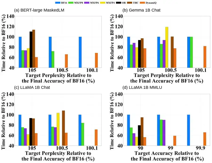
TTA, LLaMA 1B MMLU, ringTTA，LLaMA 1B MMLU，環形	72.38% (99% of BF16's 73.04%) reached about 34.5% faster than MXFP8 and 40.8% faster than BF16達到 72.38%（BF16 的 73.04% 的 99%）比 MXFP8 快約 34.5%、比 BF16 快 40.8%
TTA, Gemma 1B Chat, ringTTA，Gemma 1B Chat，環形	18% faster than MXFP8, 28% faster than MXFP6; THC, OmniReduce and MXFP4 never beat BF16比 MXFP8 快 18%、比 MXFP6 快 28%；THC、OmniReduce 與 MXFP4 都沒有贏過 BF16
Final accuracy, four workloads最終精度，四種工作負載	Within 0.1% of BF16; the other schemes lost up to 2.5%與 BF16 相差不到 0.1%；其他方法最多損失 2.5%
Overhead額外負擔	Small for DynamiQ; THC's Hadamard transform took up to 42% of a round (LLaMA 1B)DynamiQ 很小；THC 的 Hadamard 轉換最多占一個回合的 42%（LLaMA 1B）
Shared network, three other jobs共用網路，另有三個任務	Lead over MXFP8 grew from 16% to 21.5% (Gemma) and from 34.5% to 40.2% (LLaMA MMLU)領先 MXFP8 的幅度從 16% 增為 21.5%（Gemma），從 34.5% 增為 40.2%（LLaMA MMLU）
Butterfly, LLaMA 1B MMLUButterfly，LLaMA 1B MMLU	12.0% faster than MXFP8 to 99% of BF16, 37.8% to 99.5%; final accuracy 73.04% (as BF16) vs 72.86% for MXFP8達到 BF16 的 99% 比 MXFP8 快 12.0%，達到 99.5% 快 37.8%；最終精度 73.04%（與 BF16 相同），MXFP8 為 72.86%

The paper's Figure 4 (below) shows the time-to-target results for all four workloads at three targets each.

論文的 Figure 4（下圖）畫出四種工作負載、各三個目標下達到目標所需的時間。

Four grouped bar charts of time relative to BF16 at three targets each, for seven compression schemes. — Figure 4 of the paper: time to reach each target, relative to uncompressed BF16 (100%), on the 4-worker testbed with ring all-reduce (measured; MXFP6 and MXFP4 times are the paper's best-case estimates, because the A6000 lacks those formats). A missing bar means the scheme never reached that target. At the strictest target (right group in each panel) DynamiQ finishes in all four workloads, in about 65–82% of BF16's time; MXFP8 finishes in two.論文圖 4：在 4 個 worker、環形 all-reduce 的測試平台上，達到每個目標所需時間相對未壓縮 BF16（100%）的比例（實測；MXFP6 與 MXFP4 的時間是論文的最佳情況估計，因為 A6000 不支援這兩種格式）。缺少長條代表該方法始終沒有達到目標。在最嚴格的目標（每個面板最右一組），DynamiQ 在四種工作負載都完成，所需時間約為 BF16 的 65–82%；MXFP8 只完成兩種。Han, Vargaftik, Mitzenmacher and Ben Basat, SIGCOMM 2026, Figure 4 (arXiv 2602.08923 HTML; legend and panels re-arranged 2 × 2, panel titles re-typed from the sub-captions).

The average error over training on the ring explains these results (Table 3 of the paper, vNMSE):

環形上整個訓練過程的平均誤差，解釋了這些結果（論文 Table 3，vNMSE）：

Method方法	BERT-large	LLaMA 1B Chat	Gemma 1B Chat	LLaMA 1B MMLU
DynamiQ	0.00217	0.00149	0.00122	0.00096
MXFP8	0.00591	0.00320	0.00308	0.00299
MXFP6	0.02332	0.01350	0.01458	0.01298
MXFP4	0.12080	0.11059	0.11583	0.09039
OmniReduce	0.15499	0.08044	0.04676	0.04530
THC	0.00897	0.11978	0.15168	0.19599

OmniReduce relies on sparse gradients, which dense fine-tuning gradients are not. The bit-budget ablation (Diagram D) explains the default of 5 bits: below it, accuracy fell; above it, accuracy did not improve while throughput dropped.

OmniReduce 依賴稀疏的梯度，而稠密的微調梯度並不稀疏。位元預算的消融實驗（示意圖 D）說明了預設 5 位元的理由：低於它精度下降；高於它精度不再提升，吞吐量卻下降。

Diagram D. Table 4 of the paper, measured on the 4-worker ring: error against throughput for DynamiQ at 3–6 bits and for MXFP8 (8.5 bits). At 5 bits, DynamiQ is both more accurate and faster than MXFP8 on both workloads.示意圖 D。論文 Table 4，在 4 個 worker 的環上量得：DynamiQ 在 3–6 位元與 MXFP8（8.5 位元）的誤差對吞吐量。在 5 位元時，DynamiQ 在兩種工作負載上都比 MXFP8 更準確也更快。Drawn for this primer from Han et al., SIGCOMM 2026, §5.1 and Table 4 (measured).

Question問題	Calculation算式	Result結果
vNMSE, MXFP8 over DynamiQ, LLaMA MMLU (Table 3)vNMSE，MXFP8 除以 DynamiQ，LLaMA MMLU（Table 3）	$0.00299 \div 0.00096$	$\approx 3.1\times$ 2.1–3.1× over the four workloads四種工作負載為 2.1–3.1 倍
Rounds per second, 5 bits over MXFP8, LLaMA MMLU每秒回合數，5 位元除以 MXFP8，LLaMA MMLU	$2.604 \div 2.123$	$\approx 1.23\times$ Gemma: 1.09×Gemma：1.09 倍
vNMSE, ring over butterfly, DynamiQ (Tables 3, 5)vNMSE，環形除以 butterfly，DynamiQ（Table 3、5）	$0.00096 \div 0.00067$	$\approx 1.43$ MXFP8: 1.47MXFP8：1.47

The paper's results for more than four workers (2–64 workers, and 8,192 on synthetic data) and its study of how much each technique cuts the error come from simulation; this page reports no numbers from them.

論文中超過四個 worker 的結果（2–64 個 worker，以及以合成資料模擬的 8,192 個），還有各項技術分別降低多少誤差的研究，都來自模擬；本頁不引用其中的數字。

6. Limits and open questions6. 限制與未解的問題

The authors note: fine-tuning only; much larger data-parallel groups need a larger budget or butterfly or hierarchical aggregation; error growth with path length is future work. A careful reader should add:

作者指出：只做了微調；資料平行群組大很多時需提高預算，或改用 butterfly 或階層式聚合；誤差隨路徑長度的成長留待未來研究。細心的讀者還應該補上：

The measured path is short: four workers. The discussion says the testbed covers data-parallel sizes up to 64, but those runs are in the simulation section.量到的路徑很短：只有四個 worker。討論中說測試平台涵蓋到 64 的資料平行規模，但那些結果在模擬一節。
A slow network: 100 Gb/s for two GPUs. That newer GPUs keep communication a bottleneck is argued, not measured.網路偏慢：兩顆 GPU 共用 100 Gb/s。新一代 GPU 上通訊仍是瓶頸，只是論證，沒有量測。
No pre-training, FSDP or MoE run; compatibility is argued, not shown.沒有預訓練、FSDP 或 MoE 的實驗；相容性只有論證，沒有展示。
A second collective per step: the lightweight all-reduce is latency-bound; its $\alpha$ cost on small buckets is not reported.每步多一次集體操作：輕量 all-reduce 受延遲限制；它在小梯度桶上的 $\alpha$ 成本沒有報告。
Small inconsistencies: Gemma's isolated lead over MXFP8 is 18% in §5.1 and 16% in §5.2; the stated 2.5–3× lower vNMSE than MXFP8 is 2.1–3.1× in Table 3.小的不一致：Gemma 單獨執行時領先 MXFP8 的幅度在 §5.1 是 18%，在 §5.2 是 16%；文中說 vNMSE 比 MXFP8 低 2.5–3 倍，Table 3 算出來是 2.1–3.1 倍。

7. How it connects7. 與其他內容的關聯

ZipCCL is the lossless answer: no error, but an all-to-all instead of a ring and at most 1.45× fewer bytes. DynamiQ keeps the ring and sends 5 bits instead of 16.ZipCCL 是無損的答案：沒有誤差，但以 all-to-all 取代環，位元組最多只少 1.45 倍。DynamiQ 保留環形，以 5 位元取代 16 位元。
Deep dive, section 9.2: Swing and Trivance choose the aggregation shape on a torus; Appendix B shows that the shape also sets the error, and compressed sums on those shapes are untested.第 4 章第 9.2 節：Swing 與 Trivance 決定環面上的聚合形狀；附錄 B 顯示形狀也決定誤差，而在那些形狀上傳送壓縮的和還沒有人測試。
DynamiQ targets the data-parallel gradient all-reduce (Chapter 3). Llama 3 and MegaScale run data parallelism over the slowest links, and Rail-only shows that this traffic leaves the high-bandwidth domain.DynamiQ 針對資料平行的梯度 all-reduce（第 3 章）。Llama 3 與 MegaScale 讓資料平行跑在最慢的鏈路上，Rail-only 則顯示這類流量會離開高頻寬網域。

Key numbers關鍵數字

Number	數字	Meaning and setup
≈ 20% / 30%	Super-groups with norms orders of magnitude below the median (first gradient, LLaMA 1B / Gemma 1B)	範數比中位數小好幾個數量級的超群組（第一個梯度，LLaMA 1B / Gemma 1B）
5 → 4.3125 bits	Budget per coordinate → left for values after metadata (analysis)	每座標預算 → 扣掉中繼資料後留給量化值（分析）
$T_{2,4} = \tfrac{17}{512}T_{4,8}$	Threshold ratio from "one more bit, 4× less error" (analysis)	由「多一位元、誤差降為四分之一」得到的門檻比例（分析）
34.5% · 40.8%	Faster to 99% of BF16 accuracy than MXFP8 · than BF16 (LLaMA 1B MMLU, ring, 4 workers)	達到 BF16 精度 99% 比 MXFP8 · 比 BF16 快（LLaMA 1B MMLU，環形，4 個 worker）
0.00096 vs 0.00299	vNMSE, DynamiQ vs MXFP8 (LLaMA 1B MMLU, ring)	vNMSE，DynamiQ 對 MXFP8（LLaMA 1B MMLU，環形）
2.604 vs 2.123	Rounds per second, DynamiQ at 5 bits vs MXFP8	每秒回合數，5 位元的 DynamiQ 對 MXFP8
$O(n^3)$ vs $O(n^2)$	Error bound, ring vs butterfly (analysis)	誤差上界，環形對 butterfly（分析）

Terms used on this page本頁用到的術語

Multi-hop all-reduce: An all-reduce whose partial sums pass through other workers.; 部分和會經過其他 worker 的 all-reduce。
Group, super-group: 16 and 256 consecutive gradient entries that share a scale and a bit width.; 共用一個尺度與一個位元寬度的 16 個與 256 個連續梯度元素。
Lightweight all-reduce: The small first all-reduce of each super-group's mean and squared norm.; 先對每個超群組的平均值與平方範數做的小型 all-reduce。
Stochastic rounding: Random rounding to one of the two nearest levels so that the expected value is exact.; 隨機捨入到最近的兩個量化階之一，使期望值正確。
Correlated rounding: Shared randomness, $u_i = (\pi_i + \gamma_i)/n$ , that makes rounding errors of workers cancel.; 以共用亂數 $u_i = (\pi_i + \gamma_i)/n$ 讓各 worker 的捨入誤差互相抵消。
vNMSE: Squared error of the result divided by the squared norm of the true result.; 結果的平方誤差除以真實結果的平方範數。
MXFP8: A microscaling format: 8-bit E4M3 elements with one shared scale per 32 elements.; 一種微縮放格式：8 位元 E4M3 元素，每 32 個元素共用一個尺度。