Research digest 12 of 16 · Chapter 4: Collective communication

研究導讀 12 / 16 · 第 4 章：集體通訊

ZipCCL: Efficient Lossless Data Compression of Communication Collectives for Accelerating LLM TrainingZipCCL：以高效無損資料壓縮加速 LLM 訓練的集體通訊

SIGCOMM 2026Wenxiang Lin, Xinglin Pan, Ruibo Fan, Shaohuai Shi, Xiaowen Chu (HIT Shenzhen, HKUST (Guangzhou), HKUST) · paper論文

After reading, you can explain when lossless compression speeds up a collective: how ZipCCL codes BF16 exponents in 3 bits, keeps every sum local, and why the link's speed decides the answer.讀完後，你能說明無損壓縮何時能加速集體通訊：ZipCCL 如何用 3 位元編碼 BF16 指數、把每次加總留在本地，以及為何鏈路速度決定答案。

≈ 11 min · 1 interactive panel · 5-question quiz≈ 11 分鐘 · 1 個互動面板 · 5 題測驗Chapter 4 ↗第 4 章 ↗Jump to the quiz ↓跳到測驗 ↓

If you read nothing else

只讀這一段也可以

Lossless compression cannot change what a model learns, but general GPU compressors such as DietGPU and nvCOMP spend more time coding than they save on the wire. ZipCCL exploits near-Gaussian LLM tensors, whose BF16 exponents fall on a few values: it replaces each 8-bit exponent with a 3-bit code chosen from the tensor's standard deviation, and fuses the codec into NCCL-compatible collectives that never add compressed values. On 64 RTX A6000 GPUs, communication was up to 1.35× faster and training 1.16–1.18× faster; on 16 H800 GPUs, training was 1.13× faster. Over NVLink the same codec made the collectives slower. One model explains both: compression pays only below a break-even bandwidth set by the codec's speed.

無損壓縮不會改變模型學到的東西，但 DietGPU、nvCOMP 等通用 GPU 壓縮器花在編解碼上的時間，比在線路上省下的還多。ZipCCL 利用 LLM 張量接近高斯分布、BF16 指數集中在少數幾個值的性質：它依張量的標準差選出 3 位元編碼來取代每個 8 位元指數，並把編解碼器融入與 NCCL 相容、從不對壓縮值做加法的集體操作。在 64 顆 RTX A6000 GPU 上，通訊最多快 1.35 倍，訓練快 1.16–1.18 倍；在 16 顆 H800 GPU 上，訓練快 1.13 倍。走 NVLink 時，同一個編解碼器讓集體操作變慢。一個模型同時解釋兩者：只有在頻寬低於由編解碼器速度決定的損益平衡點時，壓縮才划算。

1. Where this paper sits1. 這篇論文的位置

The Chapter 4 counts the bytes each rank must send, $\tfrac{2(N-1)}{N}\,S$ for an all-reduce (sections 1–2). Section 9.5 notes that this bound assumes the endpoints send every bit, and names two ways below it: add in the switch (EPIC), or send fewer bits. ZipCCL takes the second way without loss.

第 4 章計算每個 rank 必須送出的位元組，all-reduce 是 $\tfrac{2(N-1)}{N}\,S$ （第 1–2 節）。第 9.5 節指出這個下限假設端點送出每一個位元，並列出兩條低於它的路：在交換器內做加法（EPIC），或送更少的位元。ZipCCL 不失真地走第二條路。

NCCL already trades bytes against latency (section 5): LL spends half of its bytes on flags so that small messages are usable sooner. Compression is the opposite trade, extra kernels and a size exchange for fewer bytes, so it wins only where bandwidth, not $\alpha$ , sets the time. $B$ below is the effective bandwidth of section 8. Section 9.5 gives ZipCCL's code and headline results; this page adds the break-even model (§5.3), the H800 measurements (§6.7), the MoE design and the switcher.

NCCL 本來就在位元組與延遲之間取捨（第 5 節）：LL 把一半的位元組花在旗標上，讓小訊息更早可用。壓縮是反方向的取捨：多跑幾個 kernel、多一次大小交換，換來更少的位元組，所以只在耗時由頻寬而非 $\alpha$ 決定的地方勝出。下文的 $B$ 是第 8 節所說的有效頻寬。第 9.5 節已介紹 ZipCCL 的編碼與主要結果；本頁補上損益平衡模型（§5.3）、H800 量測（§6.7）、MoE 設計與切換器。

2. The problem, measured2. 問題，用量測說話

Two measurements frame the paper. The data compress: on a Qwen3-A22B MoE model, the all-to-all traffic over 40,000 iterations was 1.33× its losslessly compressed size (the paper does not give this trace's hardware). But compression did not help: for Llama3-8B with FSDP, an all-gather compressed with DietGPU or nvCOMP was slower than plain NCCL, a "performance cliff".

兩項量測界定了問題。資料可以壓縮：在 Qwen3-A22B MoE 模型上，40,000 次迭代的 all-to-all 流量是無損壓縮後的 1.33 倍（論文沒有說明這份紀錄的硬體）。但壓縮沒有幫助：在使用 FSDP 的 Llama3-8B 上，以 DietGPU 或 nvCOMP 壓縮的 all-gather 比單純的 NCCL 還慢，也就是「效能懸崖」。

There are two causes (§2.4). A general compressor writes its own layout, not the collective's per-peer chunks, so a naive design splits and combines the data twice (Figure 1). And its kernels access memory poorly and launch often. The question is whether a codec inside the collective can repay its own time.

原因有兩個（§2.4）。通用壓縮器以自己的格式寫出結果，而不是集體操作的每個對等端區塊，所以樸素的設計要切分、合併資料各兩次（圖 1）。而且它的 kernel 記憶體存取不佳、啟動頻繁。問題在於：集體操作內的編解碼器能否賺回自己花掉的時間。

Figure 1. Where a general-purpose compressor loses time, after the paper's Figure 4. Its output does not follow the collective's per-peer chunks, so the naive design adds two splits and two combines. ZipCCL writes in the collective's chunk layout and adds only a size exchange.圖 1。通用壓縮器把時間花在哪裡，依論文 Figure 4 重畫。它的輸出不依照集體操作的每個對等端區塊排列，所以樸素做法多出兩次切分與兩次合併。ZipCCL 直接按集體操作的區塊配置寫出，只多一次大小交換。Drawn for this primer from Lin et al., SIGCOMM 2026, §2.4, §3 and Figure 4; the order of the naive steps is our reading.

3. The design3. 設計

3.1 A 3-bit exponent code, chosen from $\sigma$ 3.1 依 $\sigma$ 選出的 3 位元指數編碼

A BF16 value has 1 sign bit, 8 exponent bits and 7 mantissa bits. Sign and mantissa stay as one raw byte, so that array keeps a fixed stride for coalesced loads. The exponent is looked up in a set of 7 frequent values: a hit becomes a 3-bit code from 001 to 111; a miss becomes code 000, with the full exponent in a separate list of zero-points (escapes). A coded value needs 11 bits (8 for sign and mantissa, 3 for the code) instead of 16, a ratio of at most $16/11 \approx 1.45\times$ .

BF16 值有 1 個符號位元、8 個指數位元與 7 個尾數位元。符號與尾數保留成一個原樣的位元組，讓這個陣列維持固定步距，以便合併載入。指數則在一組 7 個常見值中查找：命中就變成 001 到 111 的 3 位元編碼；未命中就變成編碼 000，完整指數另存到 zero-point（逃逸值）清單。一個編碼後的值需要 11 位元（符號與尾數 8 位元、編碼 3 位元）而非 16 位元，壓縮比最多 $16/11 \approx 1.45$ 倍。

The 7 values come from a formula, not a histogram. Let $x$ be the unbiased exponent, so $|v| \in [2^x, 2^{x+1})$ , and assume $N(0, \sigma^2)$ . The share of values in a window of 7 binades that starts at $x$ is

這 7 個值來自公式，而不是直方圖。設 $x$ 為去偏指數，即 $|v| \in [2^x, 2^{x+1})$ ，並假設數值服從 $N(0, \sigma^2)$ 。落在從 $x$ 開始、跨 7 個二進位區間（binade）的視窗內的比例是

P_{\text{win}}(x) = \operatorname{erf}\!\Big(\frac{2^{x+7}}{\sigma\sqrt{2}}\Big) - \operatorname{erf}\!\Big(\frac{2^{x}}{\sigma\sqrt{2}}\Big)

With $u = 2^x/(\sigma\sqrt{2})$ , the condition $dP_{\text{win}}/dx = 0$ gives $128\,e^{-(128u)^2} = e^{-u^2}$ , so $(128^2 - 1)\,u^2 = \ln 128$ and $u \approx 0.0172$ . Solved for $x$ :

令 $u = 2^x/(\sigma\sqrt{2})$ ，條件 $dP_{\text{win}}/dx = 0$ 得出 $128\,e^{-(128u)^2} = e^{-u^2}$ ，所以 $(128^2 - 1)\,u^2 = \ln 128$ ， $u \approx 0.0172$ 。解出 $x$ ：

x_{\text{opt}} = \log_2 \sigma + \tfrac{1}{2}\log_2\!\Big(\frac{14 \ln 2}{16383}\Big) \approx \log_2 \sigma - 5.35

One call of torch.std gives $\sigma$ , and the code table follows with no counting or sorting (Figure 2).

呼叫一次 torch.std 得到 $\sigma$ ，不必計數或排序就得到編碼表（圖 2）。

Figure 2. Exponents of BF16 values drawn from

N(0, \sigma^2)

, our calculation for

\log_2 \sigma = 0

, in percent per binade. The 7 binades from the integer nearest

x_{\text{opt}}

hold 97.5% of the values, as in the paper's Table 1; the other 2.5% take the escape code.圖 2。取自

N(0, \sigma^2)

的 BF16 值的指數分布，是我們在

\log_2 \sigma = 0

下的計算，以每個 binade 的百分比表示。從最接近

x_{\text{opt}}

的整數開始的 7 個 binade 涵蓋 97.5% 的數值，與論文 Table 1 相同；其餘 2.5% 使用逃逸編碼。Drawn for this primer from the Gaussian model of Lin et al., SIGCOMM 2026, §4.1 (Eqs. 1–5) and Table 1; bar heights are erf differences that we computed.

Real tensors are less ideal. The paper does not break the measured 1.33× down, so the last row is our estimate:

真實張量沒有這麼理想。論文沒有拆解量到的 1.33 倍，所以最後一列是我們的估計：

Question問題	Calculation算式	Result結果
Bits per value, Gaussian case: 11, plus 8 per escape每值位元數，高斯情形：11，每個逃逸值再加 8	$11 + 8 \times 0.025$	$\approx 11.2$ bits位元
Ratio, Gaussian case壓縮比，高斯情形	$16 \div 11.2$	$\approx 1.43\times$
Bits per value at the measured 1.33×量到 1.33 倍時的每值位元數	$16 \div 1.33$	$\approx 12.0$ bits位元more escapes, padding, indices逃逸值較多，加上補齊與索引

The kernels follow the collective's layout: chunks padded to 128 bytes, the 3-bit codes stored as three aligned 1-bit arrays, a column-major shared-memory layout that cuts bank conflicts from 32-way to 4-way, and cp.async with register double buffering on Ampere GPUs.

kernel 依集體操作的配置設計：區塊補齊到 128 位元組；3 位元編碼存成三個對齊的 1 位元陣列；共享記憶體採用 column-major 配置，把 bank conflict 從 32 路降到 4 路；在 Ampere GPU 上以 cp.async 與暫存器雙緩衝隱藏延遲。

3.2 Collectives that never add compressed values3.2 從不對壓縮值做加法的集體操作

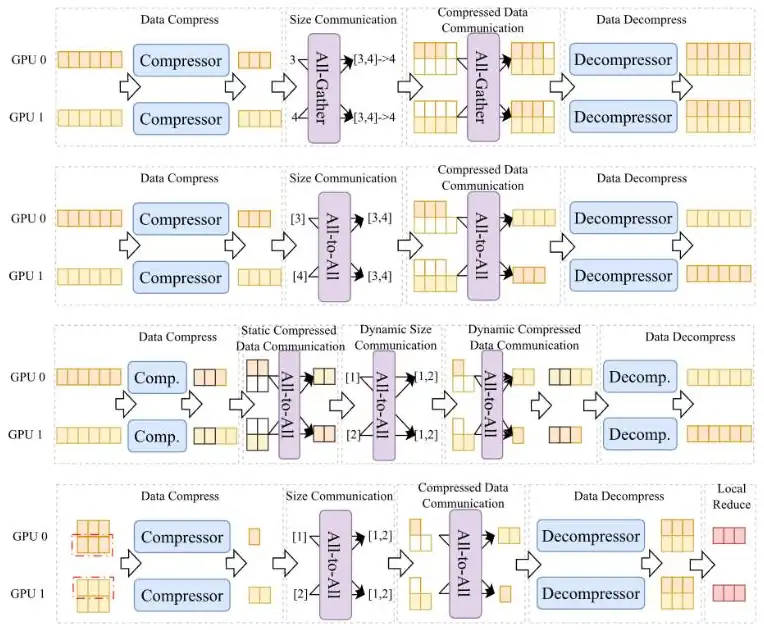
Each zipped collective is one NCCL-compatible call built on NCCL. Compressed sizes depend on the data, so each first exchanges the sizes. All-reduce is a reduce-scatter plus an all-gather, so it needs no own version. The paper's Figure 5 (below the list) draws all four workflows.

每個壓縮版集體操作都是一個建在 NCCL 之上、與 NCCL 相容的呼叫。壓縮後大小取決於資料，所以每個都先交換大小。all-reduce 就是 reduce-scatter 加 all-gather，不需要自己的版本。論文的 Figure 5（清單下方）畫出全部四種流程。

zipcclAllGather: compress the shard, all-gather the sizes (one integer per worker), all-gather the blocks, decompress all.zipcclAllGather：壓縮分片，對大小做 all-gather（每個 worker 一個整數），再對區塊做 all-gather，最後全部解壓縮。
zipcclAlltoAll: Design 1 sends sizes, then data. Design 2 first sends the static part, whose size is known before compression (the sign-mantissa array and the three code arrays), then the sizes and data of the dynamic part (the zero-points).zipcclAlltoAll：設計 1 先送大小，再送資料。設計 2 先送壓縮前就知道大小的靜態部分（符號尾數陣列與三個編碼陣列），再送動態部分（zero-point）的大小與資料。
zipcclReduceScatter: a zipcclAlltoAll, then local decompression and a sum in high precision. Inside a ring, every step would have to decompress before adding. With no addition in flight, the data can travel in BF16 even where the reduce-scatter would use FP32.zipcclReduceScatter：先做 zipcclAlltoAll，再在本地解壓縮並以高精度加總。若放在環裡，每一步都得先解壓縮才能相加。傳輸途中不做加法，所以即使 reduce-scatter 原本用 FP32，資料也能以 BF16 傳送。

Four workflow rows for two GPUs, each with compress, size communication, compressed data communication and decompress stages. — Figure 5 of the paper: how ZipCCL builds its collectives (a design diagram; top to bottom: AllGather, AlltoAll Design 1, AlltoAll Design 2, ReduceScatter). Every collective first exchanges the compressed sizes, so receivers can size their buffers; none of them ever adds compressed values, which is why reduce-scatter becomes an all-to-all followed by a local sum.論文圖 5：ZipCCL 如何組出各種集體通訊（設計示意圖；由上到下：AllGather、AlltoAll 設計 1、AlltoAll 設計 2、ReduceScatter）。每種集體通訊都先交換壓縮後的大小，讓接收端能配置緩衝區；它們從不對壓縮後的數值做加法，所以 reduce-scatter 變成先 all-to-all、再在本地相加。Lin et al., SIGCOMM 2026, Figure 5 (arXiv 2604.27844 HTML).

On a network with high bisection bandwidth, the native reduce-scatter can still win. So an adaptive switcher measures $\alpha$ and $\beta$ of both paths at start-up and compares

在對分頻寬高的網路上，原生 reduce-scatter 仍可能勝出。所以自適應切換器在啟動時量測兩條路徑的 $\alpha$ 與 $\beta$ ，並比較

T_{\mathrm{RS}}(d) = \alpha_{\mathrm{RS}} + \beta_{\mathrm{RS}}\, d, \qquad T_{\mathrm{A2A}}(d) = \alpha_{\mathrm{A2A}} + \beta_{\mathrm{A2A}}\, e\, s\, d

where $d$ is the data size, $e$ the compression factor (compressed over original size) and $s$ the precision factor (0.5 for FP32 against BF16). It compresses only when $T_{\mathrm{A2A}} \lt T_{\mathrm{RS}}$ .

其中 $d$ 是資料大小， $e$ 是壓縮係數（壓縮後大小除以原始大小）， $s$ 是精度係數（FP32 對 BF16 時為 0.5）。只有在 $T_{\mathrm{A2A}} \lt T_{\mathrm{RS}}$ 時才壓縮。

Design 2 exists for MoE. Experts receive unequal numbers of tokens, so GPUs start the all-to-all at different times. With Design 1, early GPUs can only swap sizes while they wait; with Design 2 they move most of the bytes (Figure 3).

設計 2 是為 MoE 而生。各專家收到的 token 數不同，所以各 GPU 開始 all-to-all 的時間也不同。用設計 1 時，早完成的 GPU 在等待中只能交換大小；用設計 2 時，它們能搬走大部分位元組（圖 3）。

Figure 3. The paper's 4-GPU example (§5.1), with illustrative times: one unit moves

x

bytes. GPU 1 finishes last. With sizes first, each early GPU still moves

5x

after GPU 1 is ready; with the static part first, only GPU 1's

3x

remains.圖 3。論文的 4 GPU 例子（§5.1），時間是示意值：一個單位搬

x

位元組。GPU 1 最後完成。先交換大小時，GPU 1 就緒後每顆早完成的 GPU 仍要搬

5x

；先送靜態部分時，只剩 GPU 1 的

3x

。Drawn for this primer from Lin et al., SIGCOMM 2026, §5.1 and Figure 8; the 3x and 5x volumes are the paper's, the timing is ours.

3.3 When compression pays: the break-even model3.3 壓縮何時划算：損益平衡模型

The camera-ready version adds a model (§5.3). Let $d$ be the message size per GPU, $B$ the effective bandwidth of the bottleneck link, $N$ the GPU count and $G$ the memory-bound codec throughput. An all-gather compresses only its $1/N$ shard but decompresses everything; an all-to-all codes its whole buffer both ways:

camera-ready 版加入一個模型（§5.3）。設 $d$ 為每顆 GPU 的訊息大小， $B$ 為瓶頸鏈路的有效頻寬， $N$ 為 GPU 數， $G$ 為受記憶體頻寬限制的編解碼吞吐量。all-gather 只壓縮自己 $1/N$ 的分片，卻要解壓縮全部；all-to-all 則整個緩衝區都要壓縮與解壓縮：

T^{\mathrm{AG}}_{\text{zip}} \approx \Big(1 + \frac{1}{N}\Big)\frac{d}{G} + e\,\frac{d}{B}, \qquad T^{\mathrm{A2A}}_{\text{zip}} \approx \frac{2d}{G} + e\,\frac{d}{B}

Against $T_{\text{nccl}} \approx d/B$ , compression wins below a break-even bandwidth:

與 $T_{\text{nccl}} \approx d/B$ 相比，壓縮只在頻寬低於損益平衡頻寬時勝出：

B^{*}_{\mathrm{AG}} = \frac{(1-e)\,G}{1 + 1/N} \;\to\; (1-e)\,G, \qquad B^{*}_{\mathrm{A2A}} = \frac{(1-e)\,G}{2}

So the codec's speed, not only its ratio, decides the result. Formats with fewer exponent bits gain less: FP8 E5M2 coded to 3 bits gives $e = 0.75$ , E4M3 gives $e \approx 0.88$ . FP8 also halves the wire volume by itself, so the window narrows; the paper argues that it does not vanish. Panel 1 lets you move each term.

所以決定結果的是編解碼器的速度，而不只是壓縮比。指數位元越少的格式，可省的越少：FP8 E5M2 編成 3 位元時 $e = 0.75$ ，E4M3 則 $e \approx 0.88$ 。FP8 本身已把線上流量減半，所以划算的範圍變窄；論文認為它不會消失。面板 1 讓你逐項調整。

Panel 1面板 1

Should this link carry compressed data?這條鏈路該傳壓縮資料嗎？

Collective集體操作

Codec (sets

G_c

G_d

e

)編解碼器（設定

G_c

、

G_d

、

e

）

Link on the H800 testbed (sets

B

N

)H800 測試平台的鏈路（設定

B

、

N

）

Effective bandwidth

B

有效頻寬

B

Compress throughput

G_c

壓縮吞吐量

G_c

Decompress throughput

G_d

解壓縮吞吐量

G_d

Compression factor

e

壓縮係數

e

GPUs

N

(all-gather only)GPU 數

N

（只影響 all-gather）

NCCL, 1 GB per GPU

NCCL，每顆 GPU 1 GB

Compressed: codec + wire

壓縮後：編解碼 + 傳輸

Speedup over NCCL

相對 NCCL 的加速

Break-even

B^*

損益平衡

B^*

The curve is Eqs. 8–9 with separate rates for compression and decompression: codec time $d/(N G_c) + d/G_d$ for all-gather and $d/G_c + d/G_d$ for all-to-all; with $G_c = G_d = G$ these are the paper's $(1 + 1/N)\,d/G$ and $2d/G$ . Green: compression pays; red: it loses. Dots: Table 2, measured with 1 GB per GPU on H800s (RDMA at the paper's effective $B$ of 49 and 10 GB/s; NVLink at 1 GB divided by NCCL's time). Hollow dot: the paper's model projection for an effective 800 Gb/s link, not a measurement. Defaults: $G = 1.25$ TB/s, the middle of the measured 1.2–1.3 TB/s, and $e = 0.73$ , which Table 2 implies (section 5). They give 1.30× for the RDMA all-gather, as measured. The paper quotes $B^* \approx 360$ GB/s (all-gather, many GPUs) and 180 GB/s (all-to-all); set $G = 1300$ and $e = 0.72$ to get them. nvCOMP-ANS uses its measured 256 and 401 GB/s and $e = 0.82$ , again implied by Table 2. Try the NVLink preset, then raise $G_c$ and $G_d$ : how fast must a codec be before compression pays on NVLink?

曲線是 Eq. 8–9，壓縮與解壓縮分開計速：all-gather 的編解碼時間為 $d/(N G_c) + d/G_d$ ，all-to-all 為 $d/G_c + d/G_d$ ；當 $G_c = G_d = G$ 時即論文的 $(1 + 1/N)\,d/G$ 與 $2d/G$ 。綠色：壓縮划算；紅色：壓縮吃虧。實心點：Table 2，在 H800 上以每顆 GPU 1 GB 量得（RDMA 位於論文給的有效 $B$ ，49 與 10 GB/s；NVLink 位於 1 GB 除以 NCCL 耗時）。空心點：論文以模型推估的有效 800 Gb/s 鏈路，不是量測。預設值： $G = 1.25$ TB/s，取實測 1.2–1.3 TB/s 的中間； $e = 0.73$ ，由 Table 2 推得（見第 5 節）。這組值在 RDMA all-gather 上得到 1.30 倍，與實測相同。論文給出的 $B^* \approx 360$ GB/s（all-gather，GPU 很多時）與 180 GB/s（all-to-all），可把 $G$ 設為 1300、 $e$ 設為 0.72 得到。nvCOMP-ANS 使用實測的 256 與 401 GB/s，以及同樣由 Table 2 推得的 $e = 0.82$ 。試試 NVLink 預設，再調高 $G_c$ 與 $G_d$ ：編解碼器要多快，壓縮在 NVLink 上才划算？

4. Implementation4. 實作

ZipCCL is a library of collectives on top of NCCL that takes NCCL's input formats, so it replaces NCCL calls directly. It runs in Megatron-LM (MoE) and TorchTitan (FSDP), with custom CUDA kernels tuned for Ampere. The paper gives no line count and no code link.

ZipCCL 是建在 NCCL 之上、沿用 NCCL 輸入格式的集體操作函式庫，所以能直接取代 NCCL 呼叫。它在 Megatron-LM（MoE）與 TorchTitan（FSDP）中執行，使用為 Ampere 調校的自訂 CUDA kernel。論文沒有給出程式碼行數或連結。

5. What was measured5. 量到了什麼

Two testbeds: 64 RTX A6000 GPUs, eight per node, on a 200 Gb/s network; and 16 H800 GPUs, eight per node, on a 400 Gb/s network (on the all-to-all path, a node's eight GPUs share one NIC). Models: DeepSeek-V3 cut to 64 experts and 4 layers, and a 16-layer Qwen3-MoE, on Megatron-LM; Llama3-8B with FSDP on TorchTitan; micro-batch 1, sequence length 1,024. Baselines: NCCL, DietGPU, and nvCOMP-ANS (H800; data cast to uint8, as nvCOMP has no BF16 mode).

兩個測試平台：64 顆 RTX A6000 GPU，每節點八顆，網路 200 Gb/s；以及 16 顆 H800 GPU，每節點八顆，網路 400 Gb/s（在 all-to-all 路徑上，一個節點的八顆 GPU 共用一張 NIC）。模型：縮減為 64 個專家、4 層的 DeepSeek-V3 與 16 層的 Qwen3-MoE，在 Megatron-LM 上執行；在 TorchTitan 上以 FSDP 訓練的 Llama3-8B；micro-batch 為 1，序列長度 1,024。基準：NCCL、DietGPU，以及 nvCOMP-ANS（H800；nvCOMP 沒有 BF16 模式，資料先轉成 uint8）。

Test (A6000 cluster)測試（A6000 叢集）	Measured實測結果
End-to-end, 64 GPUs端到端，64 顆 GPU	1.16× DeepSeek-V3, 1.16× Qwen3-MoE, 1.18× Llama3-8B (DeepSeek-V3: 1.06× at 16 GPUs)DeepSeek-V3 1.16 倍、Qwen3-MoE 1.16 倍、Llama3-8B 1.18 倍（DeepSeek-V3 在 16 顆 GPU 時為 1.06 倍）
Communication, 64 GPUs通訊，64 顆 GPU	All-to-all 1.25× and 1.24×; all-gather 1.35×. Native reduce-scatter was faster here, so the switcher kept itall-to-all 1.25 倍與 1.24 倍；all-gather 1.35 倍。這裡原生 reduce-scatter 較快，切換器保留了它
Micro-benchmarks微基準	Close to NCCL at small volumes; on average 1.36× (all-to-all) and 1.31× (all-gather)小資料量時與 NCCL 相近；平均 1.36 倍（all-to-all）與 1.31 倍（all-gather）
Against DietGPU對比 DietGPU	DietGPU slowed training; ZipCCL's throughput was 1.26–1.83× DietGPU's (Qwen3-MoE)DietGPU 讓訓練變慢；ZipCCL 的吞吐量是它的 1.26–1.83 倍（Qwen3-MoE）
Design 2 against Design 1設計 2 對比設計 1	1.25–1.37× end-to-end, 1.40–1.55× in all-to-all; Design 1 lost the whole gain端到端 1.25–1.37 倍，all-to-all 1.40–1.55 倍；設計 1 失去全部增益
Switcher, seven node and GPU layouts切換器，七種節點與 GPU 配置	Equal to the baseline in two, faster in five; 1.39× on average (Llama3-8B)兩種與基準相同，五種較快；平均 1.39 倍（Llama3-8B）

Gains grow with the GPU count because communication takes a larger share of each step; all-gather gained more than all-to-all because MoE imbalance hides part of the gain.

GPU 越多增益越大，因為通訊在每一步占的比例變大；all-gather 的增益大於 all-to-all，因為 MoE 的負載不均掩蓋了部分增益。

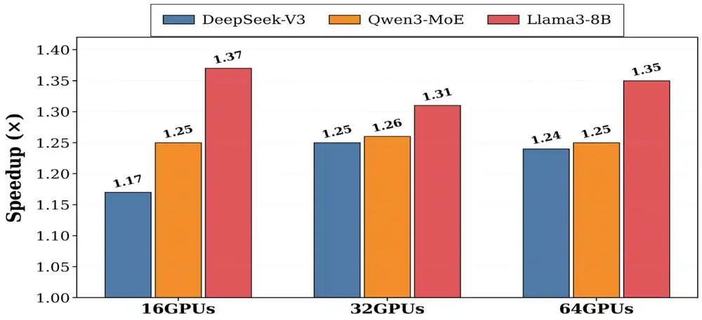
The communication speedup itself, in the paper's Figure 10 (below), stays about flat from 16 to 64 GPUs: about 1.25× for the two MoE all-to-alls and 1.31–1.37× for Llama3-8B's all-gather.

通訊本身的加速比，見論文的 Figure 10（下圖），從 16 到 64 顆 GPU 大致持平：兩個 MoE 的 all-to-all 約 1.25 倍，Llama3-8B 的 all-gather 為 1.31–1.37 倍。

Grouped bar chart of speedup for three models at 16, 32 and 64 GPUs, between 1.17 and 1.37. — Figure 10 of the paper: communication speedup of ZipCCL over NCCL on the A6000 testbed at 16, 32 and 64 GPUs (measured). DeepSeek-V3 and Qwen3-MoE use all-to-all; Llama3-8B uses all-gather. The bars range from 1.17× to 1.37×.論文圖 10：在 A6000 測試平台的 16、32、64 顆 GPU 上，ZipCCL 相對 NCCL 的通訊加速比（實測）。DeepSeek-V3 與 Qwen3-MoE 用 all-to-all；Llama3-8B 用 all-gather。長條介於 1.17 到 1.37 倍。Lin et al., SIGCOMM 2026, Figure 10 (arXiv 2604.27844 HTML).

On the 16 H800s, training was 1.13× faster on both Megatron-LM (Qwen-MoE) and TorchTitan (Llama3-8B). Without the static and dynamic split, Qwen-MoE gained only 1.06×. nvCOMP-ANS gave 0.97× (slower) and 1.04×. Table 2 of the paper then isolates the link, with 1 GB per GPU (Figure 4).

在 16 顆 H800 上，Megatron-LM（Qwen-MoE）與 TorchTitan（Llama3-8B）的訓練都快 1.13 倍。關掉靜態與動態部分的拆分後，Qwen-MoE 只快 1.06 倍。nvCOMP-ANS 得到 0.97 倍（變慢）與 1.04 倍。論文 Table 2 接著以每顆 GPU 1 GB 單獨檢視鏈路的影響（圖 4）。

Figure 4. Table 2 of the paper, measured with 1 GB per GPU on H800s (8 GPUs on NVLink, 16 on 400 Gb/s RDMA), as time relative to NCCL; the left part of each compressor's bar is compression plus decompression. The same codec time sinks both compressors on NVLink and is repaid on RDMA.圖 4。論文 Table 2，在 H800 上以每顆 GPU 1 GB 量得（8 顆 GPU 走 NVLink，16 顆走 400 Gb/s RDMA），以相對 NCCL 的時間表示；壓縮器長條的左段是壓縮加解壓縮。同樣的編解碼時間，在 NVLink 上拖垮兩個壓縮器，在 RDMA 上則被賺回。Drawn for this primer from Lin et al., SIGCOMM 2026, §6.7 and Table 2 (measured).

The codec cost, about 0.85 ms (all-gather) and 1.6 ms (all-to-all), does not depend on the link. The arithmetic from Table 2:

編解碼成本約 0.85 ms（all-gather）與 1.6 ms（all-to-all），與鏈路無關。由 Table 2 計算：

Question問題	Calculation算式	Result結果
RDMA all-gather, NCCL over ZipCCLRDMA all-gather，NCCL 除以 ZipCCL	$19.75 \div 15.17$	$\approx 1.30\times$
RDMA all-to-allRDMA all-to-all	$101.76 \div 76.71$	$\approx 1.33\times$
NVLink all-gatherNVLink all-gather	$2.92 \div 3.01$	$\approx 0.97\times$ slower變慢
NVLink all-to-allNVLink all-to-all	$2.96 \div 5.05$	$\approx 0.59\times$ slower變慢
Compression factor implied by the RDMA all-gatherRDMA all-gather 隱含的壓縮係數	$(15.17 - 0.84) \div 19.75$	$e \approx 0.73$ all-to-all: 0.74all-to-all：0.74
NVLink all-to-all without its codec timeNVLink all-to-all 扣掉編解碼時間	$5.05 - 1.61$	$3.44$ msmore than NCCL's 2.96 ms比 NCCL 的 2.96 ms 還長

On RDMA the paper measured an effective bandwidth of about 49 GB/s (all-gather) and 10 GB/s (all-to-all), and a codec throughput of 1.2–1.3 TB/s, about 5× and 3× nvCOMP-ANS's 256 and 401 GB/s. Its model then puts the break-even points near 360 and 180 GB/s and projects 1.23× and 1.30× at an effective 800 Gb/s: model outputs, not measurements.

在 RDMA 上，論文量到的有效頻寬約 49 GB/s（all-gather）與 10 GB/s（all-to-all），編解碼吞吐量為 1.2–1.3 TB/s，約為 nvCOMP-ANS 的 256 與 401 GB/s 的 5 倍與 3 倍。它的模型由此把損益平衡點定在約 360 與 180 GB/s，並推估有效 800 Gb/s 時為 1.23 倍與 1.30 倍：這些是模型輸出，不是量測。

6. Limits and open questions6. 限制與未解的問題

The paper's own rules: compress only below the break-even bandwidth (inter-node RDMA, not NVLink), not when the job is host-bound (the extra kernels and size exchange add CPU work), and expect a narrower window with FP8. A careful reader should add:

論文自己的規則：只在頻寬低於損益平衡點時壓縮（跨節點 RDMA，而非 NVLink）；任務受主機限制時不要壓縮（多出的 kernel 與大小交換會增加 CPU 負擔）；FP8 下可用範圍會變窄。細心的讀者還應該補上：

Scale. At most 64 GPUs. The node count in the setup text does not match 64 GPUs; the ablation's layouts (up to 8 nodes of 8 GPUs) mean eight nodes.規模。最多 64 顆 GPU。設定說明中的節點數與 64 顆 GPU 對不上；消融實驗的配置（最多 8 個節點、每節點 8 顆）表示共八個節點。
Communication-heavy setups. A 4-layer DeepSeek-V3 and micro-batch 1 inflate the communication share. The gain was smaller on H800s (1.13×).通訊比重偏高。4 層的 DeepSeek-V3 與大小為 1 的 micro-batch 放大了通訊比例。H800 上的增益較小（1.13 倍）。
Lossless on the wire. The compressed reduce-scatter sums in a different place and order, so it matches a native reduce-scatter only up to rounding order. No loss curves are shown.無損指的是線上的位元。壓縮版 reduce-scatter 的加總位置與順序不同，所以只在捨入順序的範圍內與原生版一致。論文沒有給出 loss 曲線。
Design 2 is partly scheduling. Starting early would also help uncompressed NCCL under imbalance; this is not tested.設計 2 有一部分是排程的功勞。負載不均時提早開始，對未壓縮的 NCCL 也有幫助；論文沒有測試。
The model is optimistic on NVLink. For the all-to-all it predicts about 3.8 ms, that is $1.6 + 0.73 \times 2.96$ ; 5.05 ms was measured.模型在 NVLink 上偏樂觀。對 all-to-all 它預測約 3.8 ms，即 $1.6 + 0.73 \times 2.96$ ；實測是 5.05 ms。
Not measured. Tensor-parallel all-reduce and pipeline send and receive.沒有量測。張量平行的 all-reduce，以及管線平行的 send 與 receive。

7. How it connects7. 與其他內容的關聯

DynamiQ is the lossy counterpart: it keeps the ring and recompresses each partial sum at every hop, so it must control the added error. ZipCCL avoids additions on the path.DynamiQ 是有損的對照：它保留環形結構，在每一跳重新壓縮部分和，所以必須控制增加的誤差。ZipCCL 則避開路徑上的加法。
Deep dive, section 9.5: EPIC adds inside switches, where ZipCCL's codes would first need decoding; Chapter 4 lists the combination as open. Section 5 and Theseus: the switcher is a run-time choice, like NCCL's auto-selection.第 4 章第 9.5 節：EPIC 在交換器內做加法，ZipCCL 的編碼在那裡得先解碼；第 4 章把兩者的結合列為未解問題。第 5 節與 Theseus：切換器是一種執行期選擇，類似 NCCL 的自動選擇。
Guided readings: Meta's RoCE fabric, Llama 3 and Alibaba HPN give each GPU about 400 Gb/s (50 GB/s), far below the break-even points. Rail-only keeps most bytes in the NVLink domain, where compression loses. MegaScale hides much communication behind compute, and only the exposed part can shrink.論文導讀：Meta 的 RoCE 網路、Llama 3 與 Alibaba HPN 給每顆 GPU 約 400 Gb/s（50 GB/s），遠低於損益平衡點。Rail-only 讓大部分位元組留在 NVLink 網域內，而壓縮在那裡吃虧。MegaScale 把大量通訊藏在計算後面，只有外露的部分能被縮短。

Key numbers關鍵數字

Number	數字	Meaning and setup
16 → 11 bits	Bits per coded BF16 value, at most a 31% saving (analysis)	每個編碼後 BF16 值的位元數，最多省 31%（分析）
1.33×	Measured all-to-all compression ratio, Qwen3-A22B	量到的 all-to-all 壓縮比，Qwen3-A22B
1.35× · 1.16–1.18×	Best communication · end-to-end speedups, 64 A6000	最大通訊加速 · 端到端加速，64 顆 A6000
1.13×	End-to-end speedup, 16 H800, 400 Gb/s	端到端加速，16 顆 H800，400 Gb/s
101.76 → 76.71 ms	RDMA all-to-all, 1 GB per GPU, 16 H800	RDMA all-to-all，每顆 GPU 1 GB，16 顆 H800
2.96 → 5.05 ms	NVLink all-to-all, 8 H800: compression loses	NVLink all-to-all，8 顆 H800：壓縮吃虧
1.2–1.3 TB/s	ZipCCL codec throughput (nvCOMP-ANS: 256 / 401 GB/s)	ZipCCL 編解碼吞吐量（nvCOMP-ANS：256 / 401 GB/s）
$(1-e)G/2$	Break-even bandwidth of an all-to-all (analysis)	all-to-all 的損益平衡頻寬（分析）

Terms used on this page本頁用到的術語

Zero-point (escape): A value whose exponent is outside the coded set: code 000, full exponent stored apart.; 指數不在編碼集合內的值：編碼為 000，完整指數另外存放。
Static and dynamic part: Compressed data whose size is known before compression, and data whose size depends on the values.; 壓縮前就知道大小的壓縮資料，以及大小取決於數值的資料。
Compression factor $e$: Compressed size over original size; about 0.69 at best for BF16 with this code.; 壓縮後大小除以原始大小；以此編碼處理 BF16 時最好約 0.69。
Codec throughput $G$: Bytes per second that the compressor or decompressor processes.; 壓縮器或解壓縮器每秒處理的位元組數。
Break-even bandwidth $B^*$: The effective bandwidth above which compression no longer speeds up a collective.; 有效頻寬高於此值時，壓縮就不再加速集體操作。
Adaptive switcher: A cost-model rule that picks compressed all-to-all plus a local sum, or the native reduce-scatter.; 以成本模型在「壓縮 all-to-all 加本地加總」與原生 reduce-scatter 之間選擇的規則。
Bank conflict: Threads of a warp using the same shared-memory bank, which serializes their accesses.; 一個 warp 的多個執行緒存取同一個共享記憶體 bank，使存取被序列化。