The step-time budget: why the network decides how far training scales步驟時間帳:為何網路決定訓練能擴展到多大
Add up the arithmetic and the bytes of one training step, see why communication takes a growing share of the step as GPUs are added, learn how overlap hides it, and see what the resulting traffic looks like on a link.把一個訓練步驟的算術與位元組加總起來,看出為何通訊在 GPU 增加時占步驟的比例越來越大、重疊如何把它藏起來,以及最後的流量在鏈路上長什麼樣子。
This chapter builds on Chapters 1, 2, 3, 4. These earlier terms appear most often below; each chip links to its definition.
本章建立在第 1、2、3、4 章之上。下列較早定義的名詞在本章最常出現;點選即可回到它的定義。
New terms in this chapter (3)本章新名詞(3)
Each term is defined in the text where it first appears; the link jumps there. Terms from earlier chapters are listed under "Before you start".
每個名詞都在它第一次出現的段落中定義,點連結可跳過去。前面各章的名詞列在「開始之前」。
- Strong scaling強擴展 Running the same job (same global batch) on more GPUs: compute per GPU falls, DP bytes per GPU do not. 在更多 GPU 上跑同一個工作(全域批次不變):每顆 GPU 的運算下降,DP 位元組不變。
- Elephant flow, low entropy大象流、低熵 A flow large enough to fill a link by itself; low entropy means few distinct flows for switches to spread. 大到能獨自塞滿一條鏈路的流;低熵指交換器可分散的不同流很少。
- Burstiness, duty cycle突發性、工作週期 Training traffic is on at full rate or off; the duty cycle is the share of a step a NIC spends sending. 訓練流量不是全速就是靜止;工作週期是 NIC 在一個步驟中傳送的時間比例。
5.1One step on a timeline時間軸上的一個步驟
Where the communication sits depends on how the model is split, which Chapter 3 covers in detail. Three kinds appear on the timeline of Figure 5.1. Tensor parallelism (TP) splits each weight matrix across the 8 GPUs of a server, so each layer needs an all-reduce in the middle of the forward pass and another in the backward pass. This traffic is on the critical path: the next layer cannot start until it finishes. Pipeline parallelism (PP) gives each group of GPUs a slice of layers and passes activations from stage to stage with point-to-point sends. Data parallelism (DP) gives each group a different part of the batch. The groups must average their gradients once per step with a reduce-scatter, and re-gather the updated parameters with an all-gather. DP traffic is the largest in bytes but happens once per step, and much of it can run while the backward pass is still computing earlier layers.
通訊落在時間線的哪裡,取決於模型怎麼切分;第 3 章會詳細討論。圖 5.1 的時間線上出現三種。張量平行(TP)把每個權重矩陣切到一台伺服器的 8 顆 GPU 上,所以每一層在前向中途需要一次 all-reduce、反向中途再一次。這種流量在關鍵路徑上:它沒完成,下一層就不能開始。管線平行(PP)給每一組 GPU 一段層,用點對點傳送把激活值一階段一階段往後傳。資料平行(DP)給每一組不同的那部分批次。各組每步必須用一次 reduce-scatter 平均梯度,再用一次 all-gather 重新收集更新後的參數。DP 流量的位元組數最大,但每步只發生一次,而且大部分可以在反向還在計算前面的層時就進行。
5.2The network roofline for one step一個步驟的網路 roofline
Figure 5.2 draws this rule for the GPU's memory and for its NIC, and Panel 5.1 applies it to one step.
圖 5.2 把這條規則畫在 GPU 的記憶體與 NIC 上,面板 5.1 則把它套用到一步上。
5.3How many bytes per step每步多少位元組
The numerator of the network roofline is the bytes each GPU must send per step. Start with the simplest layout, pure data parallelism: every GPU holds a full copy of the model and computes gradients on its own slice of the batch. The gradient has one number per parameter. In BF16 that is 2 bytes, so for 405B parameters the gradient is 810 GB on every GPU. All copies must be averaged. The standard way is a ring all-reduce: each GPU sends its gradient in pieces around a ring, first reducing (reduce-scatter) and then distributing the result (all-gather). If is the gradient size, the bytes every GPU sends and receives are
網路 roofline 的分子是每顆 GPU 每步必須送出的位元組。從最簡單的配置開始:純資料平行,每顆 GPU 持有完整的模型副本,對自己那片批次計算梯度。梯度每個參數一個數字。BF16 下是 2 位元組,所以 405B 參數的梯度在每顆 GPU 上都是 810 GB。全部 份副本必須被平均。標準做法是環狀 all-reduce:每顆 GPU 把自己的梯度切成 塊沿著環傳送,先做歸約(reduce-scatter),再把結果分發(all-gather)。若 是梯度大小,每顆 GPU 送出並收到的位元組數是
Figure 5.3 shows where the comes from on four GPUs.
圖 5.3 以四顆 GPU 說明 從哪裡來。
For any large that is just under . Now put in Llama 3 405B on 16,384 GPUs with a 16M-token batch ( tokens), taking the compute side from Section 1.2:
對任何大的 ,這剛好略小於 。現在代入 Llama 3 405B、16,384 顆 GPU、16M token 的批次( 個 token),計算這一邊取自第 1.2 節:
| Question問題 | Calculation算式 | Result結果 |
|---|---|---|
| Bytes each GPU sends and receives per step, GB每顆 GPU 每步送出並收到的位元組, GB | GBabout 1.62 TB約 1.62 TB | |
| Time on a 400 Gb/s NIC (50 GB/s)在 400 Gb/s NIC(50 GB/s)上的時間 | s | |
| Arithmetic per GPU per step ( from Section 1.2, shared by 16,384 GPUs)每顆 GPU 每步的算術量(第 1.2 節的 ,由 16,384 顆 GPU 分攤) | FLOP | |
| Compute time per step at 400 TFLOP/s以 400 TFLOP/s 計的每步計算時間 | s | |
| Communication time over compute time通訊時間與計算時間之比 | ||
| Arithmetic intensity (Section 1.1): FLOP per byte sent算術強度(第 1.1 節):每送出一個位元組的 FLOP | FLOP/Bwell below the 8,000 balance point遠低於 8,000 的平衡點 |
Each GPU moves about 1.62 TB per step, which takes about 32 seconds, while its share of the arithmetic takes about 6.2 seconds. Communication would take five times longer than computation. Pure data parallelism cannot work at this scale, whatever the network. The intensity check from Section 1.1 says the same: about 1,500 FLOP per byte, well below the 8,000 balance point.
每顆 GPU 每步搬約 1.62 TB,約需 32 秒,而它分到的算術只要約 6.2 秒。通訊會比計算多花五倍時間。在這個規模,純資料平行不可能可行,不管網路多好。第 1.1 節 的強度檢查說的是同一件事:每位元組約 1,500 FLOP,遠低於 8,000 的平衡點。
Sharding changes where the bytes go, not how many there are. With FSDP (fully sharded data parallelism, the DP that Llama 3 uses), the parameters, gradients and optimizer state are divided among the DP group. Each step then needs an all-gather to assemble the parameters before they are used and a reduce-scatter to sum the gradients afterward. Each of these moves per GPU, so the total is the same as an all-reduce, or if the parameters are re-sharded after the forward pass and gathered a second time for the backward pass, which Llama 3 avoids. The win is memory, not bandwidth. Llama 3 reduce-scatters its gradients in FP32 for numerical stability (Llama 3 §3.3.2), which doubles that leg to 4 bytes per parameter. The table collects the formulas. The pattern to notice: every data-parallel variant moves about 2 bytes per parameter per GPU per step in some combination, and nothing about adding GPUs makes that number smaller.
分片改變的是位元組去哪裡,不是有多少。使用 FSDP(完全分片資料平行,Llama 3 用的 DP)時,參數、梯度與優化器狀態分散到 DP 群組中。每步因此需要在使用參數前做一次 all-gather 把參數湊齊,之後再做一次 reduce-scatter 把梯度加總。兩者各搬 /每 GPU,所以總量與 all-reduce 一樣是 ;若參數在前向之後重新分片、反向時再收集一次,就是 ,Llama 3 避免了這一點。賺到的是記憶體,不是頻寬。Llama 3 為了數值穩定以 FP32 做梯度的 reduce-scatter(Llama 3 §3.3.2),這一段因此加倍為每個參數 4 位元組。下表整理這些公式。要注意的模式是:每一種資料平行變體都以某種組合、每顆 GPU 每步搬約每個參數 2 位元組,而增加 GPU 不會讓這個數字變小。
| Collective | 集體操作 | Bytes sent per GPU | 每顆 GPU 送出的位元組 | Used for | 用途 |
|---|---|---|---|---|---|
| all-reduce (ring) | DP gradients; TP activations inside each layer | DP 梯度;每層內的 TP 激活值 | |||
| reduce-scatter | FSDP and ZeRO-2 gradient sum | FSDP 與 ZeRO-2 的梯度加總 | |||
| all-gather | FSDP parameters; context-parallel keys and values | FSDP 參數;上下文平行的 key 與 value | |||
| send / receive | message size | 訊息大小 | PP activations between stages | 階段之間的 PP 激活值 | |
| all-to-all | Expert routing in MoE; embedding exchange in recommendation models | MoE 的專家路由;推薦模型的 embedding 交換 |
The way out is to shrink per GPU by splitting the model, which is what tensor and pipeline parallelism do. If GPUs share one copy of the model, each GPU holds parameters and its DP exchange is bytes. Llama 3's layout of and gives , and its 16,384 GPUs form such replicas:
出路是把模型切開以縮小每顆 GPU 的 ,這正是張量平行與管線平行做的事。若 顆 GPU 共用一份模型,每顆 GPU 持有 個參數,它的 DP 交換是 位元組。Llama 3 的 、 配置給出 ,它的 16,384 顆 GPU 組成 份這樣的副本:
| Question問題 | Calculation算式 | Result結果 |
|---|---|---|
| Parameters per GPU每顆 GPU 的參數 | parameters 個參數about 3.2 billion約 32 億 | |
| Their size in BF16, 2 bytes eachBF16 下的大小,每個 2 位元組 | GB | |
| DP traffic per step: ring all-reduce over the replicas, times that每步 DP 流量:在 份副本間做環狀 all-reduce,是上一列的 倍 | GB | |
| Its time on a 400G NIC (50 GB/s)在 400G NIC(50 GB/s)上的時間 | s4% of the 6.2 s of computation6.2 秒計算的 4% | |
| With the FP32 reduce-scatter: BF16 all-gather (1 share) plus FP32 reduce-scatter (2 shares)改用 FP32 reduce-scatter:BF16 all-gather(1 份)加 FP32 reduce-scatter(2 份) | GBabout 19 GB約 19 GB | |
| Its time on a 400G NIC在 400G NIC 上的時間 | s6% of the 6.2 s of computation6.2 秒計算的 6% | |
| Arithmetic intensity with the FP32 reduce-scatter: FLOP per byte sent用 FP32 reduce-scatter 時的算術強度:每送出一個位元組的 FLOP | FLOP/Bfar above 8,000遠高於 8,000 |
So each GPU holds about 3.2 billion parameters, 6.3 GB in BF16, and its DP traffic drops to about 12.6 GB per step, 0.25 s on a 400G NIC, or about 19 GB and 0.38 s with the FP32 reduce-scatter. Against 6.2 s of computation that is 4–6%, and most of it can be hidden. The intensity is now about 130,000 FLOP per byte, far above 8,000. But the split is not free. It creates the TP all-reduce inside every layer and the PP sends between stages. The order [TP, CP, PP, DP] that Llama 3 uses (§3.3.2) is a bandwidth order. The traffic that is largest per second and sits on the critical path, TP, gets NVLink inside the server. PP, which is small, gets the network inside a group of racks. DP, which is large per step but happens once per step and can be fetched ahead of time, is the only kind allowed over the slowest links between those groups (Chapter 6). Chapter 3 works through each dimension; here you only need the volumes.
所以每顆 GPU 持有約 32 億參數、BF16 下 6.3 GB,它的 DP 流量降到約每步 12.6 GB、在 400G NIC 上 0.25 秒;若用 FP32 reduce-scatter 則約 19 GB、0.38 秒。相對 6.2 秒的計算,這是 4–6%,而且大部分可以被隱藏。強度現在約為每位元組 130,000 FLOP,遠高於 8,000。但切分不是免費的。它製造出每一層內的 TP all-reduce 與階段之間的 PP 傳送。Llama 3 使用的 [TP, CP, PP, DP] 順序(§3.3.2)是一個頻寬順序。每秒流量最大且在關鍵路徑上的 TP,拿到伺服器內的 NVLink。很小的 PP,拿到一群機櫃內部的網路。每步很大、但每步只發生一次且可預先抓取的 DP,是唯一被允許走這些群組之間最慢鏈路的那一種(第 6 章)。第 3 章逐一處理每個維度;這裡你只需要流量大小。
Panel 5.2 computes this exchange for any split, group size and precision.
面板 5.2 對任何切分、群組大小與精度計算這次交換。
Alibaba's HPN paper gives measured volumes for one step of GPT-3 175B at , , on 32K GPUs (HPN Table 3): tensor parallelism 560 MB in all-reduce and all-gather, data parallelism 5.5 GB in all-reduce, pipeline parallelism 6 MB in send and receive. Two of these you can now reproduce:
Alibaba 的 HPN 論文給出 GPT-3 175B 在 、、、32K 顆 GPU 下一步的實測流量(HPN Table 3):張量平行在 all-reduce 與 all-gather 中 560 MB,資料平行在 all-reduce 中 5.5 GB,管線平行在 send 與 receive 中 6 MB。其中兩個你現在可以自己算出來:
| Question問題 | Calculation算式 | Result結果 |
|---|---|---|
| Per-GPU shard: 175B parameters over GPUs每顆 GPU 的分片:175B 參數分給 顆 GPU | parameters 個參數 | |
| That shard in BF16: the DP message on each GPU該分片在 BF16 下的大小:每顆 GPU 的 DP 訊息 | GBHPN: 5.5 GBHPN:5.5 GB | |
| Pipeline message: one micro-batch of activations, 管線訊息:一個 micro-batch 的激活值, | MBHPN: 6 MBHPN:6 MB |
The 5.5 GB is the data-parallel message size on each GPU, and the 6 MB is one micro-batch crossing a stage boundary. The ratio is about 1,000 : 100 : 1. HPN arranges jobs the other way round from Llama 3: it keeps TP and DP inside one large group of racks and lets only the 6 MB of PP traffic cross its slowest links (HPN §7; Chapter 6). Both arrangements follow the same rule. The thinnest link gets the traffic that is either tiny or tolerant of delay.
5.5 GB 就是每顆 GPU 上資料平行的訊息大小,6 MB 則是一個 micro-batch 跨越階段邊界。比例約為 1,000 : 100 : 1。HPN 安排任務的方向和 Llama 3 相反:把 TP 與 DP 留在一大群機櫃之內,只讓 6 MB 的 PP 流量跨越它最慢的鏈路(HPN §7;第 6 章)。兩種安排遵循同一條規則。最細的鏈路拿到的流量,要嘛極小、要嘛能忍受延遲。
Bytes per GPU, by dimension每顆 GPU 的位元組,依維度
HPN's Table 3, re-read重讀 HPN 的 Table 3
HPN's Table 3 (below) gives message sizes for GPT-3 175B at TP8-PP8-DP512. The DP entry reproduces exactly: 175B parameters spread over the 64 GPUs (TP8 × PP8) of one replica leave parameters per GPU, which at 2 bytes each is 5.5 GB (the formula is in the table). The PP entry reproduces for a micro-batch of one 2,048-token sequence split across 8 TP ranks: 6.3 MB. The TP entry, 560 MB, does not follow from a whole step (tens of gigabytes); it is the size of one layer's collectives for a few sequences. Read it as "one collective of each kind": per message, and PP, smallest and most tolerant, is the only traffic allowed on the 15:1 core links (HPN §7).
HPN 的 Table 3(下表)給出 GPT-3 175B 在 TP8-PP8-DP512 下的訊息大小。DP 那格可以精確重現:175B 參數分到一個副本的 64 顆 GPU(TP8 × PP8)上,每顆 GPU 有 個參數,每個 2 位元組就是 5.5 GB(算式見下表)。PP 那格在一條 2,048 token 序列的 micro-batch、切到 8 個 TP rank 時重現:6.3 MB。TP 那格的 560 MB 無法從一整步推出(那會是數十 GB);它的大小相當於一層的集體操作處理幾條序列。把它讀成「每種集體操作各一次」:每則訊息 ,而最小、最能忍的 PP 是唯一被允許走 15:1 核心鏈路的流量(HPN §7)。
| Dimension | 維度 | Collective (HPN) | 集體操作(HPN) | HPN Table 3 | HPN Table 3 | Our formula | 我們的公式 | Match | 吻合度 |
|---|---|---|---|---|---|---|---|---|---|
| TP | AllReduce / AllGather | 560 MB | 352 MB per layer per 2K-token micro-batch (ring) | same order; unit not stated | 同一數量級;單位未說明 | ||||
| DP | AllReduce | 5.5 GB | exact (message size) | 精確(訊息大小) | |||||
| PP | Send / Recv | 6 MB | exact for , | 、 時精確 |
Press the HPN preset in Panel 5.3, then raise EP to 64 with top-. The all-to-all bytes land near the DP bytes, but on the critical path of every MoE layer and between servers. Which link in Chapter 6 carries them?
在面板 5.3 按下 HPN 預設組,再把 EP 拉到 64、top-。all-to-all 位元組落在 DP 位元組附近,但位在每個 MoE 層的關鍵路徑上、還跨伺服器。第 6 章的哪條鏈路承載它們?
5.4The communication share grows with the cluster通訊占比隨叢集變大而增加
Write the two halves of the step as formulas. With GPUs, a global batch of tokens, and FLOP/s achieved per GPU, the compute time is . With a model-parallel group of , the DP group is and the communication time is , where is the NIC bandwidth in bytes per second:
把一步的兩半寫成公式。有 顆 GPU、全域批次 個 token、每顆 GPU 實際達到 FLOP/s 時,計算時間是 。模型平行群組為 時,DP 群組是 ,通訊時間是 , 是 NIC 頻寬(位元組/秒):
Now fix and grow . This is strong scaling: the same job on more machines. falls as . hardly moves: for the factor is already above 0.87, so , a constant set by the model size, the layout and the NIC. The communication share therefore rises steadily, and so does its effect on utilization. Doubling the cluster halves the compute time and leaves the exchange where it was.
現在固定 、增加 。這是強擴展(strong scaling):同一個任務放到更多機器上。 以 下降。 幾乎不動: 時 已經超過 0.87,所以 ,是一個由模型大小、配置與 NIC 決定的常數。通訊比例 因此穩定上升,它對使用率的影響也一樣。叢集加倍,計算時間減半,交換量留在原地。
Figure 5.4 applies the two formulas to the layout of Llama 3 at five cluster sizes.
圖 5.4 把這兩個公式套用到 Llama 3 的配置與五種叢集大小。
Software can hide part of behind . Overlap means issuing a collective for one part of the model while the GPU computes another part. The reduce-scatter of layer 's gradients runs while the backward pass works on layer . The all-gather of the next layer's parameters runs during the current layer's forward. Pipeline sends are posted asynchronously. If a fraction of the communication is overlapped, the exposed part is and the step takes . Two limits apply. Hidden communication cannot exceed the compute it hides behind, so when is larger than , as in pure data parallelism, no amount of overlap saves you. And overlap assumes the network delivers the bytes before the compute runs out. A link that carries two flows at once delivers each at half rate. The collective that depended on it now finishes late, the compute that was supposed to cover it has ended, and the remainder is exposed. Worse, the rank that was waiting starts its next phase late, and every rank that depends on it waits in turn. This is why jitter, small random variation in delay, in the network is more damaging than its average bandwidth suggests. Overlap converts a bandwidth problem into a deadline, and deadlines are missed by the tail, not by the mean.
軟體可以把一部分 藏在 後面。重疊(overlap)是指在 GPU 計算模型的某一部分時,為另一部分發出集體操作。第 層梯度的 reduce-scatter 在反向處理第 層時執行。下一層參數的 all-gather 在這一層的前向期間執行。管線傳送以非同步方式提交。若通訊中有 的比例被重疊,暴露的部分是 ,一步耗時 。有兩個限制。被隱藏的通訊不能超過它所藏身的計算,所以當 大於 ——例如純資料平行——再多重疊也救不了你。而且重疊假設網路在計算用完之前把位元組送到。一條同時承載兩條流的鏈路對每條只以一半速率送達。依賴它的集體操作現在晚完成,本來要掩護它的計算已經結束,剩下的部分就暴露了。更糟的是,等待中的那個 rank 會晚開始下一階段,依賴它的每個 rank 又接著等。這就是為什麼網路的抖動(延遲中小而隨機的變化)比它的平均頻寬所暗示的更具破壞性。重疊把頻寬問題變成一個期限,而期限是被尾端錯過的,不是被平均值錯過的。
Animation 5.1 plays one step on one GPU, with one gradient bucket per layer. Switch the link to half rate to see the deadline missed.
動畫 5.1 播放單顆 GPU 上的一步,每層一個梯度桶。把鏈路切到半速,看期限如何被錯過。
ByteDance's MegaScale paper is the cleanest published measurement of this curve. Training a 175B model, MegaScale reaches 65.3% MFU on 256 GPUs and 55.2% on 12,288: a 48× increase in GPUs for a 10-point fall. Standard Megatron-LM on the same hardware falls from 53.0% to 41.2% (MegaScale Table 2). Both systems do the same arithmetic per token. The difference is how much communication each leaves exposed. MegaScale overlaps in all three dimensions and gains 6.2 MFU points from overlap alone in its ablation (TP 2.2, PP 2.5, DP 1.5). Because the exposed part grows with scale, its advantage grows too, from 1.23× at 256 GPUs to 1.34× at 12,288. Llama 3 shows the same slope more gently. Doubling from 8,192 to 16,384 GPUs at the same sequence length moved MFU from 43% to 41% (Llama 3 Table 4), because DP doubled from 64 to 128 while TP and PP, which carry the exposed traffic, stayed fixed.
ByteDance 的 MegaScale 論文是這條曲線最乾淨的公開量測。訓練一個 175B 模型時,MegaScale 在 256 顆 GPU 上達到 65.3% MFU、在 12,288 顆上 55.2%:GPU 增加 48 倍,下降 10 個百分點。同樣硬體上的標準 Megatron-LM 從 53.0% 降到 41.2%(MegaScale Table 2)。兩個系統每個 token 做同樣的算術。差別在於各自暴露了多少通訊。MegaScale 在三個維度都做重疊,消融實驗中單靠重疊就多了 6.2 個 MFU 百分點(TP 2.2、PP 2.5、DP 1.5)。因為暴露的部分隨規模增長,它的優勢也隨之增長,從 256 顆 GPU 的 1.23 倍到 12,288 顆的 1.34 倍。Llama 3 以較緩的斜率顯示同樣的現象。在相同序列長度下從 8,192 加倍到 16,384 顆 GPU,MFU 從 43% 降到 41%(Llama 3 Table 4),因為 DP 從 64 加倍到 128,而承載暴露流量的 TP 與 PP 維持不變。
Figure 5.5 plots these measured points.
圖 5.5 畫出這些實測點。
Take the Llama 3 numbers in Panel 5.4 below (405B parameters, 16,384 GPUs, 16M-token batch) and set the model-parallel group to 1. How much of the step is now communication, and what does the MFU estimate become? Set it back to 128 and halve the network bandwidth. Why does the MFU barely move? Then raise the GPU count to 131,072 and watch which term wins.
在下面的面板 5.4 裡取 Llama 3 的數字(405B 參數、16,384 顆 GPU、16M token 批次),把模型平行群組設為 1。現在一步裡有多少是通訊?MFU 估計變成多少?把它設回 128 並把網路頻寬減半。為什麼 MFU 幾乎不動?再把 GPU 數拉到 131,072,看看哪一項勝出。
5.5Mixture-of-experts: hiding the all-to-all混合專家:把 all-to-all 藏起來
Both systems hide the all-to-all behind compute, and the worked example shows why they must. DeepSeek-V3's DualPipe schedule pairs a forward chunk with a backward chunk. The attention and MoE compute of one micro-batch then runs while the MoE all-to-all of another is in flight (technical report §3.2.1; ISCA §4.2). Up to 20 SMs of each H800 run the communication: they forward between IB and NVLink, move data between buffers, reduce the combine and cast types (ISCA §4.4.1). The paper does not state the communication share of a step, because DualPipe hides it. The full job ran at 19.926 s per step, of which 2.06 s was pipeline bubble, at 43.73% MFU (ISCA Table 4, measured; non-causal FLOP count).
兩個系統都把 all-to-all 藏在計算後面,而上面的算例說明了為什麼非這樣不可。DeepSeek-V3 的 DualPipe 排程把一個正向 chunk 和一個反向 chunk 配成一對。於是一個 micro-batch 的注意力與 MoE 計算在執行時,另一個 micro-batch 的 MoE all-to-all 正在傳送(技術報告 §3.2.1;ISCA §4.2)。每顆 H800 最多用 20 個 SM 執行通訊:在 IB 與 NVLink 之間轉送、在緩衝區之間搬資料、做合併的歸約,以及型別轉換(ISCA §4.4.1)。論文沒有給出通訊占一步的比例,因為 DualPipe 把它藏住了。完整任務每步 19.926 秒,其中 2.06 秒是管線氣泡,MFU 為 43.73%(ISCA Table 4,實測;以非因果方式計算 FLOP)。
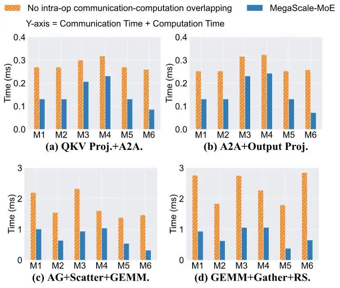
MegaScale-MoE does not need a second micro-batch. It writes the forward and backward passes of a whole MoE layer as explicit operators and runs communication on separate CUDA streams beside independent compute (inter-operator overlap, §4.1). It also fuses each all-to-all with its GEMM: computed tiles go to remote GPUs at once, a signal per tile tells the receiver, and a small number of SMs do the all-to-all (intra-operator overlap, §4.2). On 240 H800 GPUs, SP + EP gave 1.13× Megatron-LM's throughput, inter-operator overlap 1.22× and the fused kernels 1.28× (Table 5, measured). The fused kernels cut the time of each communication-and-compute pair 1.2–4.7× (Figure 5.6). Before such work, communication was 43.6% of the forward time of ByteDance's internal model on Hopper GPUs (MegaScale-MoE §1, setup not given). MegaScale-MoE also notes that DualPipe needs twice the parameters in memory (MegaScale-MoE §8).
MegaScale-MoE 不需要第二個 micro-batch。它把整個 MoE 層的正向與反向寫成明確的運算子,讓通訊在獨立的 CUDA stream 上、與互不相依的計算並行(運算子間重疊,§4.1)。它也把每個 all-to-all 和對應的 GEMM 融合:算好的 tile 立刻送往遠端 GPU,每個 tile 一個訊號通知接收端,並只用少數幾個 SM 做 all-to-all(運算子內重疊,§4.2)。在 240 顆 H800 上,SP + EP 的吞吐是 Megatron-LM 的 1.13 倍,加上運算子間重疊為 1.22 倍,再加上融合 kernel 為 1.28 倍(Table 5,實測)。融合 kernel 讓每一對通訊與計算的時間縮短 1.2–4.7 倍(圖 5.6)。在這些改進之前,字節跳動內部模型在 Hopper GPU 上的通訊占正向時間的 43.6%(MegaScale-MoE §1,未說明設定)。MegaScale-MoE 也指出 DualPipe 需要兩倍的參數記憶體(MegaScale-MoE §8)。
MegaScale-MoE gives a simple model for this limit (MegaScale-MoE §7, model). The ratio of expert compute to EP communication is about
MegaScale-MoE 為這個上限給了一個簡單的模型(MegaScale-MoE §7,模型)。專家計算與 EP 通訊的比值約為
where is the width of one expert, the link bandwidth and the peak FLOP rate. The all-to-all can hide only if . does not depend on the number of experts, on top- or on the hidden size. For on an H800 (989 TFLOP/s), is about 9.9 on 400 GB/s NVLink but only about 1.2 on a 50 GB/s NIC. For the small experts of DeepSeekMoE () it is about 1.0 even on NVLink (our arithmetic). So small experts and faster GPUs push EP toward the fastest link. Panel 5.5 puts the NIC time, the NVLink time and the compute time of one MoE layer on one axis. Its defaults are the worked example above; the MegaScale-MoE preset keeps EP inside the node.
其中 是一個專家的寬度, 是鏈路頻寬, 是峰值 FLOP 速率。只有 時 all-to-all 才藏得住。 與專家數、top- 或隱藏維度都無關。在 H800(989 TFLOP/s)上取 ,走 400 GB/s 的 NVLink 時 約 9.9,走 50 GB/s 的 NIC 時只有約 1.2。DeepSeekMoE 的小專家()即使走 NVLink 也只有約 1.0(我們的計算)。所以小專家與更快的 GPU 會把 EP 推向最快的鏈路。面板 5.5 把一個 MoE 層的 NIC 時間、NVLink 時間與計算時間放在同一條軸上。預設值就是上面的算例;MegaScale-MoE 預設組把 EP 留在節點內。
Skew inside each call每次呼叫內的偏斜
Balance on average still leaves skew in each call. FAST profiled Megatron-LM MoE pre-training with 32 experts, one per GPU. Some GPU pairs exchanged more than 12 times the median volume, and the bytes of one pair changed by orders of magnitude from call to call (Figure 5.7, measured). An all-to-all ends when the busiest NIC finishes. So its time is the largest row or column sum of the server-level traffic matrix, not the mean, and large skewed transfers overload the links into the busiest receivers (FAST §2–§3). Neither MoE system reports skew numbers for its own training run.
平均上平衡了,每次呼叫仍有偏斜。FAST 剖析了 Megatron-LM 的 MoE 預訓練(32 個專家、每顆 GPU 一個)。有些 GPU 對交換的量超過中位數的 12 倍,同一對 GPU 的位元組數在呼叫之間相差好幾個數量級(圖 5.7,實測)。all-to-all 要等最忙的 NIC 做完才結束。所以它的時間是伺服器層級流量矩陣中最大的列和或行和,而不是平均值;大而偏斜的傳輸也會讓通往最忙接收端的鏈路超載(FAST §2–§3)。兩個 MoE 系統都沒有報告自己訓練時的偏斜數字。
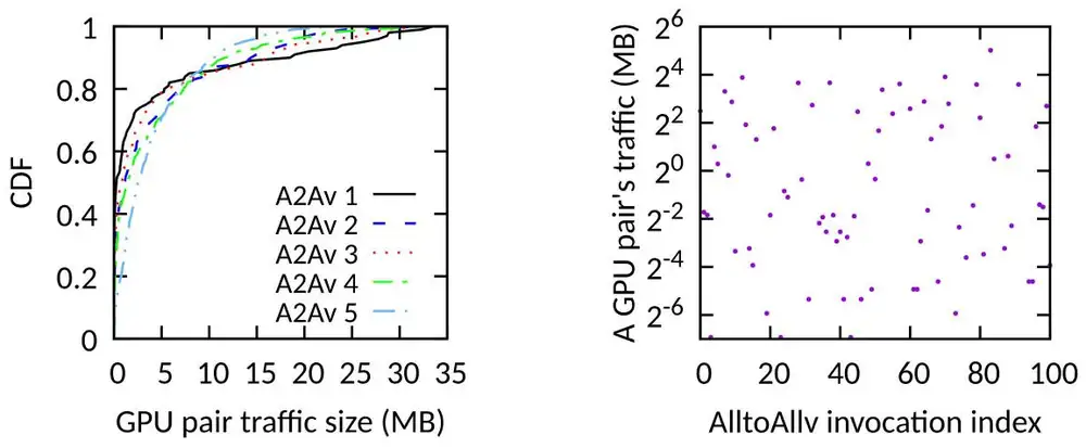
FAST answers with a schedule computed at every call. It first evens out the bytes per NIC by moving data over the scale-up network. Then it splits the server-level matrix into one-to-one stages, a Birkhoff decomposition: no NIC receives from two senders at once, and the busiest server works in every stage. On 4 servers of 8 H200 GPUs, with one 400 Gb/s InfiniBand NIC per GPU, it was 1.2–1.3× faster than NCCL on skewed loads (Zipf 0.8) and equal on balanced loads. The host CPU computes the schedule in 25 µs for 32 GPUs (FAST §5, measured). Theseus (SIGCOMM 2026) makes the schedule itself a run-time variable, so that all GPUs can switch to a new schedule as MoE loads shift. The collectives research page covers both.
FAST 的對策是每次呼叫都重新計算排程。它先經 scale-up 網路搬移資料,讓每張 NIC 的位元組數相等。再把伺服器層級的矩陣拆成一對一的階段,也就是 Birkhoff 分解:沒有任何 NIC 同時從兩個發送端接收,而最忙的伺服器每個階段都在工作。在 4 台、每台 8 顆 H200、每顆 GPU 一張 400 Gb/s InfiniBand NIC 的環境中,偏斜負載(Zipf 0.8)下它比 NCCL 快 1.2–1.3 倍,平衡負載下兩者相同。主機 CPU 為 32 顆 GPU 計算排程只要 25 µs(FAST §5,實測)。Theseus(SIGCOMM 2026)把排程本身變成執行期的變數,讓所有 GPU 能隨 MoE 負載的移動切換到新的排程。集體通訊研究前沿頁涵蓋這兩者。
5.6What the traffic looks like on the wire流量在線路上長什麼樣
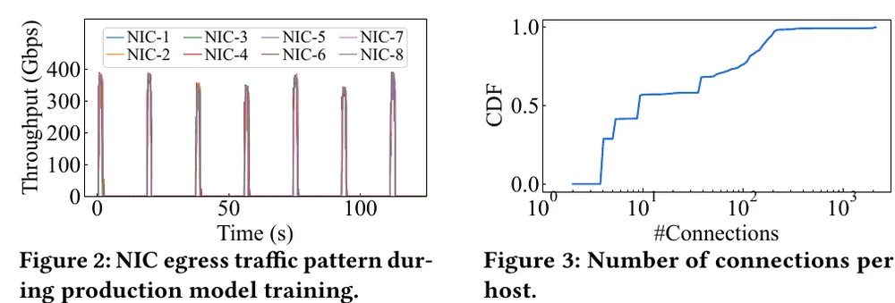
Put the previous sections together and you can predict the traffic without measuring it. Every GPU computes for seconds, then its NIC sends its share of the exchange at full line rate for seconds, then goes quiet. Every GPU in the job does this at the same moment, because they all finished the same backward pass on the same batch. Alibaba measured exactly this on a production host (HPN Figure 2, our Figure 5.8): each of the eight NICs jumps to about 400 Gb/s, holds it, and drops to zero until the next step. The same paper counted connections (HPN Figure 3): a training host has tens of them, where a host in an ordinary cloud workload has thousands. Meta's measurement is finer still (Meta RoCE Table 2): on 128 GPUs an all-reduce opens about 4 RDMA connections, called queue pairs, per GPU, and an all-to-all about 15. Meta gives the three properties the names that this book uses throughout: low entropy (few distinct flows, so a switch has little variety to spread over its links), burstiness (on at line rate or off, switching at millisecond scale), and elephant flows (one flow fills a 400 Gb/s link by itself).
把前面幾節合起來,不用量測也能預測流量。每顆 GPU 計算 秒,然後它的 NIC 以滿線速送出自己那份交換、持續 秒,然後安靜下來。任務中每顆 GPU 都在同一時刻做這件事,因為它們都剛對同一批資料完成同一個反向傳播。Alibaba 在生產主機上量到的正是這個(HPN Figure 2,即本章圖 5.8):八張 NIC 的每一張都跳到約 400 Gb/s、維持住、然後降到零直到下一步。同一篇論文數了連線數(HPN Figure 3):訓練主機只有幾十條,一般雲端工作負載的主機則有數千條。Meta 的量測更細(Meta RoCE Table 2):在 128 顆 GPU 上,一次 all-reduce 每顆 GPU 約開 4 條 RDMA 連線,稱為 queue pair,一次 all-to-all 約 15 條。Meta 給這三個特性的名字貫穿本書:低熵(不同的流很少,交換器能拿來分散到各鏈路上的變化很少)、突發(要嘛滿線速、要嘛關閉,以毫秒尺度切換)、大象流(一條流自己就能塞滿一條 400 Gb/s 鏈路)。
Animation 5.2 plays two steps of one NIC, then zooms out to one 15-second counter sample.
動畫 5.2 播放一張 NIC 的兩步,再拉遠到一個 15 秒的計數器樣本。
A web data center is the opposite on every axis, and the opposite is what its network was designed for. A front-end server has thousands of flows, most of them a few kilobytes, starting and ending at unrelated times. Their sum is smooth because of the law of large numbers: if independent flows each contribute a share with relative standard deviation , the total has relative standard deviation . A million flows average out to a load that barely moves. Two flows do not average at all. Chapter 8 shows how this difference breaks the usual way in which switches spread traffic over their links.
網頁資料中心在每一個軸上都相反,而它的網路正是為那個相反面設計的。一台前端伺服器有數千條流,多數只有幾 KB,在互不相關的時刻開始與結束。它們的總和很平滑,因為大數法則:若 條獨立的流各貢獻一份、相對標準差為 ,總和的相對標準差是 。一百萬條流平均成一個幾乎不動的負載。兩條流完全不會平均。第 8 章說明這個差異如何破壞交換器把流量分散到各鏈路上的一般做法。
Three consequences follow, and later chapters take them up. First, buffers. When two bursts share one link, the link receives twice what it can carry for the length of a burst. The excess is burst length × line rate: a 50 ms burst at 400 Gb/s is 2.5 GB, far more than the tens of megabytes in a single-chip switch (Section 2.8). It must be dropped or stopped at the source. Second, loss. RDMA NICs recover badly from a lost packet, so training networks try never to drop one (Chapter 7). Third, separation. Storage reads, checkpoint writes and logging have their own bursts: a Llama 3 checkpoint is 1 MB to 4 GB per GPU, written by 16,000 GPUs at once. If that traffic shared the GPU network, a checkpoint could stall a collective, so Meta and Alibaba give it a separate network (Chapter 9). Alibaba keeps storage there even though the GPU network has eight times the bandwidth, because mixing the two made training performance fluctuate (HPN §8). The panel below shows the burst shape and the buffering it implies.
三個後果隨之而來,後面的章節會處理。第一,緩衝。兩個突發共用一條鏈路時,鏈路在整段突發期間收到它能承載的兩倍。多出來的量是突發長度 × 線速:400 Gb/s 下 50 ms 的突發是 2.5 GB,遠多於單晶片交換器的幾十 MB 緩衝(第 2.8 節)。它必須被丟掉,或在來源端被停住。第二,丟包。RDMA NIC 從丟包恢復的代價很高,所以訓練網路盡量一個封包都不丟(第 7 章)。第三,分離。儲存讀取、檢查點寫入與日誌有自己的突發:Llama 3 的檢查點每顆 GPU 1 MB 到 4 GB,由 16,000 顆 GPU 同時寫入。如果那些流量與 GPU 網路共用,一次檢查點就可能讓集體操作停住,所以 Meta 與 Alibaba 都讓它走另一個網路(第 9 章)。Alibaba 即使 GPU 網路有八倍的頻寬,仍把儲存留在那裡,因為兩者混用讓訓練效能出現波動(HPN §8)。下面的面板顯示突發的形狀以及它所隱含的緩衝需求。
In Panel 5.6, keep the average load fixed by moving the duty cycle and the line rate together (for example 25% at 400 Gb/s, then 50% at 200 Gb/s). The average does not change. Which tiles do, and what does that say about sizing a network by average utilization?
在面板 5.6 中,同時調整工作週期與線速以維持平均負載不變(例如 400 Gb/s 下 25%,再改成 200 Gb/s 下 50%)。平均值不變。哪些格子變了?這對「用平均使用率來規劃網路」說明了什麼?
5.7What changes if如果改變了什麼
The formulas of Chapter 3 and this chapter answer a designer's "what if". If the next GPU has 141 or 192 GB of HBM, PP can drop from 16 to 8 for the same model: twice the TP bytes per GPU, still on NVLink, and half the bubble if the DP degree and the batch per replica stay fixed (with the GPU count fixed instead, the bubble barely moves). If the batch doubles, DP bytes per step are unchanged, TP, PP and EP bytes double, and the bubble halves. If the model becomes MoE, a data-dependent all-to-all appears in every MoE layer (Figure 3.15). It needs either a network layer that joins GPUs of different local ranks, as HPN keeps, or a scale-up domain that does the copying, as in the two production systems of Section 3.8 (Chapter 6). If the sequence grows to 128K, CP takes GPUs from DP (Figure 5.9) and exposes all-gathers in every attention layer. Each is a change in the traffic matrix before it is a change in the network. Panel 5.7 applies the first two changes to the layout of Section 3.7.
第 3 章與本章的公式回答設計者的「如果」。如果下一代 GPU 有 141 或 192 GB 的 HBM,同一個模型的 PP 可以從 16 降到 8:每顆 GPU 的 TP 位元組加倍,仍在 NVLink 上;若 DP 度數與每個副本的批次不變,氣泡減半(若改為固定 GPU 數,氣泡幾乎不動)。如果批次加倍,每步的 DP 位元組不變,TP、PP 與 EP 的位元組加倍,氣泡減半。如果模型變成 MoE,每個 MoE 層出現依資料而定的 all-to-all(圖 3.15)。它需要一層連接不同本地 rank 之 GPU 的網路(如 HPN 所保留的),或一個替它做這種複製的 scale-up 域(如第 3.8 節的兩個生產系統;第 6 章)。如果序列長到 128K,CP 從 DP 拿走 GPU(圖 5.9),並讓每個注意力層的 all-gather 暴露。每一項都先是流量矩陣的改變、然後才是網路的改變。面板 5.7 把前兩項改變套用到第 3.7 節的配置上。
A step is fixed arithmetic plus exchanges whose bytes per GPU do not shrink with scale. With pure data parallelism a GPU would move about 2 × 810 GB per step for Llama 3 405B, far longer than its compute; splitting the model 128 ways cuts that to about 12.6 GB. At a fixed batch, compute time falls as 1/G while the exchange time stays flat, so the exchange's share grows with the cluster: this is strong scaling, and it is why MFU falls with size. Overlap hides an exchange as long as each chunk's communication finishes before its computation; MoE systems need it most, because their all-to-all is large against little compute per token. On the wire, training traffic is a few very large flows that burst to line rate in lockstep and then idle, the opposite of web traffic.
一個步驟是固定的算術,加上每顆 GPU 位元組數不隨規模縮小的交換。以 Llama 3 405B 為例,純資料平行時一顆 GPU 每步約要搬 2 × 810 GB,遠比它的計算時間長;把模型切成 128 份後降到約 12.6 GB。批次固定時,計算時間隨 1/G 下降,交換時間卻幾乎不變,所以交換所占比例隨叢集變大而增加:這就是強擴展,也是 MFU 隨規模下降的原因。只要每一塊的通訊都在它的計算結束前完成,重疊就能把交換藏起來;MoE 系統最需要這一點,因為它們的 all-to-all 相對於每個 token 的少量計算而言很大。在線路上,訓練流量是少數幾條非常大的流,同步地衝到線速、然後閒置,與網頁流量正好相反。
Chapter 6 begins Part II, the network itself: how switches are wired together so that thousands of GPUs can exchange these bytes.
第 6 章開始第二部,談網路本身:交換器如何連接起來,讓數千顆 GPU 能交換這些位元組。