Research digest 6 of 16 · Chapter 4: Collective communication

研究導讀 6 / 16 · 第 4 章：集體通訊

ResCCL: Resource-Efficient Scheduling for Collective CommunicationResCCL：集體通訊的資源高效排程

SIGCOMM 2025Tongrui Liu, Chenyang Hei, Fuliang Li et al. (Northeastern University, SIAT CAS, Alibaba Cloud) · paper論文

After reading, you can explain why one thread block per connection wastes SMs and link time, and how ResCCL schedules primitives and shares thread blocks to fix it.讀完後，你能說明為何每條連線配一個 thread block 會浪費 SM 與鏈路時間，以及 ResCCL 如何排程原語並共用 thread block 來解決。

≈ 10 min · 1 interactive panel · 5-question quiz≈ 10 分鐘 · 1 個互動面板 · 5 題測驗Chapter 4 ↗第 4 章 ↗Jump to the quiz ↓跳到測驗 ↓

If you read nothing else

只讀這一段也可以

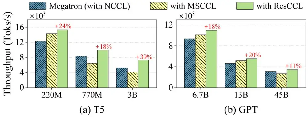
Collective libraries give every GPU-to-GPU connection its own thread block (TB), run an algorithm one micro-batch at a time, and interpret custom schedules. On A100 servers this was costly: extra-channel TBs were idle 98.2% of the time, TBs were blocked up to 67.1%, a TACCL AllReduce used 31.8% of the active link bandwidth, and interpretation cost 17.1%. ResCCL compiles the algorithm offline: one TB runs the same primitive for every micro-batch, connections never active together share a TB, and plain kernels replace the interpreter. With the same algorithms as MSCCL on 16–32 A100 GPUs, it measured up to 2.5× MSCCL's bandwidth with 20–78% fewer TBs, and up to 39% more Megatron-LM throughput than with NCCL.

集體通訊函式庫給每條 GPU 對 GPU 的連線一個專屬的 thread block（TB），一次一個 micro-batch 地執行演算法，並直譯自訂排程。在 A100 伺服器上代價很高：額外 channel 的 TB 有 98.2% 的時間閒置，TB 最多 67.1% 的時間卡住，一個 TACCL AllReduce 只用到 31.8% 的活躍鏈路頻寬，直譯損失 17.1%。ResCCL 離線編譯演算法：一個 TB 對每個 micro-batch 執行同一個原語，從不同時活躍的連線共用一個 TB，並以單純的 kernel 取代直譯器。在 16–32 顆 A100 GPU 上執行與 MSCCL 相同的演算法，它量到最多 MSCCL 2.5 倍的頻寬、少 20–78% 的 TB，Megatron-LM 吞吐比用 NCCL 時最多高 39%。

1. Where this paper sits1. 這篇論文的位置

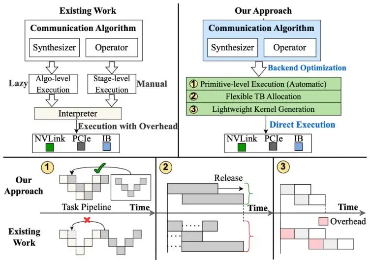
Section 4.5 shows that each channel is one CUDA thread block on its own SM, with its own buffer and connection; section 9.1 shows solvers such as TACCL and TE-CCL that write algorithms for a runtime such as MSCCL. Those works decide which chunk crosses which link, and when. ResCCL decides how a given algorithm runs on the GPU: which thread block executes which primitive, and when.

第 4.5 節說明每個 channel 是一個在自己 SM 上的 CUDA thread block，有自己的緩衝區與連線；第 9.1 節介紹 TACCL、TE-CCL 等為 MSCCL 這類執行環境寫演算法的求解器。那些工作決定哪個 chunk 何時經過哪條鏈路。ResCCL 決定一個既定的演算法如何在 GPU 上執行：哪個 thread block 何時執行哪個原語。

The paper's terms (§2.1): each TB runs a kernel made of primitives (send, recv, recvReduceCopy); a chunk is what one operation moves, about 1% of the data. A micro-batch is the data of one execution of the algorithm, so a large buffer runs as $n$ micro-batches; it is not the training micro-batch. Existing backends run at algorithm level, one micro-batch after another, or at stage level, with manual stages on their own TBs and buffers (MSCCLang).

論文的用語（§2.1）：每個 TB 執行一個由原語（send、recv、recvReduceCopy）組成的 kernel；chunk 是一次操作搬動的量，約為資料的 1%。micro-batch 是演算法執行一次所搬的資料，所以大緩衝區要跑 $n$ 個 micro-batch；它不是訓練用的 micro-batch。現有的 backend 以演算法層級執行（一個 micro-batch 接一個），或以階段層級執行（手動階段各有自己的 TB 與緩衝區，MSCCLang）。

2. The problem, measured2. 問題，用量測說話

The authors measured four costs of existing runtimes on A100 servers with 200 Gb/s RoCE (§2.2):

作者在使用 200 Gb/s RoCE 的 A100 伺服器上，量到現有執行環境的四種代價（§2.2）：

Bubbles. Link utilization falls as servers are added (Figure 1). A TACCL AllReduce on two servers used 31.8% of the active link bandwidth, because fast NVLink transfers wait for slow inter-node ones.氣泡。伺服器變多時鏈路使用率下降（圖 1）。兩台伺服器上的 TACCL AllReduce 只用到 31.8% 的活躍鏈路頻寬，因為快速的 NVLink 傳輸要等慢速的跨節點傳輸。
Idle extra channels. In a single-node expert AllReduce, the TBs of additional channels were idle 98.2% of the time.閒置的額外 channel。在單節點的專家設計 AllReduce 中，額外 channel 的 TB 有 98.2% 的時間閒置。
Blocked TBs. With one TB per connection, TBs waited on synchronization with slower links for up to 67.1% of their time.被卡住的 TB。每條連線一個 TB 時，TB 最多有 67.1% 的時間在等較慢鏈路的同步。
Interpretation. Re-reading the algorithm and per-step routing at run time cost 17.1% on average, against a kernel that runs directly.直譯。執行時重新讀取演算法與每一步的路由，與直接執行的 kernel 相比平均損失 17.1%。

One more measurement shapes the design: on one NIC, P2P bandwidth rose with the TB count up to 4 and fell at 8 (Figure 4 of the paper; no values given). Past the link's capacity, extra TBs only contend, so a TB should be a time slot on a link, not a fixture of a connection.

還有一項量測決定了設計方向：在一張 NIC 上，P2P 頻寬隨 TB 數增加到 4 個為止，到 8 個時下降（論文 Figure 4，未給數值）。超過鏈路容量後，多的 TB 只會互相爭用，所以 TB 應該是鏈路上的一個時間槽，而不是綁死在連線上的固定配備。

Figure 1. Global link utilization of existing algorithms on their existing runtimes, from Table 1 of the paper (measured, A100 servers, 200 Gb/s RoCE). Rows: servers × GPUs per server. AG and AR: AllGather and AllReduce. The outlined cell is the TACCL AllReduce at 31.8%.圖 1。現有演算法在現有執行環境上的整體鏈路使用率，取自論文 Table 1（實測，A100 伺服器、200 Gb/s RoCE）。列：伺服器數 × 每台 GPU 數。AG 與 AR：AllGather 與 AllReduce。框起來的格子是 31.8% 的 TACCL AllReduce。Drawn for this primer from Liu et al., SIGCOMM 2025, Table 1.

3. The design3. 設計

ResCCL is an offline compiler plus a runtime. An expert writes the algorithm in ResCCLang as Transfer(srcRank, dstRank, step, chunkId, opType) operations on per-rank buffers cut into chunks, where opType is send, recv or recvReduceCopy; channels and TBs are derived, not written. The compiler analyzes dependencies, schedules primitives, allocates TBs and generates kernels.

ResCCL 是一個離線編譯器加上一個執行環境。專家用 ResCCLang 把演算法寫成一串 Transfer(srcRank, dstRank, step, chunkId, opType) 操作，作用在每個 rank 切成 chunk 的緩衝區上，opType 是 send、recv 或 recvReduceCopy；channel 與 TB 由編譯器推導，不必手寫。編譯器依序分析相依、排程原語、配置 TB，並產生 kernel。

Figure 1 of the ResCCL paper: existing work runs an algorithm at algorithm or stage level through an interpreter; ResCCL adds primitive-level execution, flexible thread-block allocation and lightweight kernel generation, with three timeline sketches — Figure 1 of the paper (a design diagram). Left: existing backends run an algorithm lazily or in manual stages, through an interpreter. Right: ResCCL adds primitive-level execution (1), flexible TB allocation (2) and generated kernels (3); the sketches below show each one over time.論文的 Figure 1（設計示意圖）。左：現有 backend 以惰性方式或手動階段、透過直譯器執行演算法。右：ResCCL 加上原語層級執行 (1)、彈性 TB 配置 (2) 與產生的 kernel (3)；下方草圖畫出每個機制隨時間的樣子。Screenshot of Liu et al., SIGCOMM 2025, Figure 1 (p. 2).

3.1 A cost model for three granularities3.1 三種粒度的成本模型

An algorithm is a set of transfer tasks: one chunk on one link, with its dependencies. The busiest link sets the time, $T_{\text{algo}} = \max_i T_i$ . For $n$ micro-batches of $m$ tasks, with start-up cost $\alpha$ , chunk size $c$ , inverse bandwidth $\beta$ and bubble $B_j$ of task $j$ , the paper compares (§3):

一個演算法是一組傳輸任務：一條鏈路上的一個 chunk，加上它的相依關係。最忙的鏈路決定耗時， $T_{\text{algo}} = \max_i T_i$ 。對 $n$ 個各有 $m$ 個任務的 micro-batch，啟動成本 $\alpha$ 、chunk 大小 $c$ 、頻寬倒數 $\beta$ 、任務 $j$ 的氣泡 $B_j$ ，論文比較的是（§3）：

\begin{aligned} T_A &= n \sum_{j=1}^{m} \big(\alpha + c\beta + B_j\big) \\ T_S &= \max_{k} \; n \sum_{j=1}^{m_k} \big(z_k(\alpha + c\beta) + \gamma L(z_k) + B_j\big) \\ T_P &= t_{\text{Load}} + n\,m\,(\alpha + c\beta) + n \sum_{j=1}^{m'} B_j \end{aligned}

Algorithm level ( $T_A$ ) pays every bubble in every micro-batch. Stage level ( $T_S$ ) runs stages in parallel, but a stage can put $z_k$ times a link's capacity of threads on it, with contention penalty $\gamma L(z_k)$ . Task level ( $T_P$ ) fills a pipeline once and keeps only the $m' \le m$ bubbles that scheduling cannot remove (Figure 2). For large $n$ , task level wins. The paper asserts $m' \ll m$ without measuring it; optimal scheduling is NP-hard, so ResCCL uses a heuristic.

演算法層級（ $T_A$ ）在每個 micro-batch 都付出所有氣泡。階段層級（ $T_S$ ）讓各階段平行執行，但一個階段可能在鏈路上放 $z_k$ 倍於鏈路容量的執行緒，爭用懲罰為 $\gamma L(z_k)$ 。任務層級（ $T_P$ ）只填一次管線，之後只留下排程消除不了的 $m' \le m$ 個氣泡（圖 2）。 $n$ 很大時任務層級勝出。論文斷言 $m' \ll m$ 但沒有量測；最佳排程是 NP-hard，所以 ResCCL 用啟發式方法。

Figure 2. The three granularities for four micro-batches (colours), each sent on NVLink, then over the slower NIC, then forwarded on NVLink. Algorithm level leaves links idle, while stage level overlaps micro-batches but can put two of them on one link at once (outlined in red), and task level overlaps them without sharing. The durations are chosen to show the pattern.圖 2。三種粒度下的四個 micro-batch（以顏色區分），各自先在 NVLink 上送、再經較慢的 NIC、再在 NVLink 上轉送。演算法層級讓鏈路閒置，階段層級讓 micro-batch 重疊，但可能讓兩個同時用一條鏈路（紅框處），任務層級則重疊而不共用。時間長度是為了呈現這個模式而設定的。Drawn for this primer from Liu et al., SIGCOMM 2025, §2.1 and §3, Eqs. 3–5.

3.2 Schedule tasks, not micro-batches3.2 排程任務，而不是 micro-batch

Dependency analysis builds a DAG of tasks. An edge is a data dependency: two tasks touch the same buffer offset, so their order is fixed for correctness; such edges exist only within one chunk. Tasks on one link at overlapping times have a communication dependency: correct, but slow together. Across micro-batches only communication dependencies remain.

相依分析把任務建成一個 DAG。邊代表資料相依：兩個任務存取同一個緩衝區位移，為了正確性順序必須固定；這種邊只存在於同一個 chunk 之內。在重疊時間使用同一條鏈路的任務之間有通訊相依：一起執行是正確的，但很慢。跨 micro-batch 時只剩通訊相依。

HPDS (hierarchical priority-based dynamic scheduling) packs tasks into sub-pipelines (Figure 3). Chunks wait in a priority queue, less-used first. HPDS takes the top chunk, adds every task with no pending data dependency and no link conflict, lowers the chunk's priority by one, and moves on; when no chunk can add a task, the sub-pipeline closes. Inter-machine latency was at least 2.5× intra-machine latency, so an intra-node task never joins the sub-pipeline of the inter-node task it depends on. Each TB then runs its task for all $n$ micro-batches. On 8 GPUs in two servers, HPDS was up to 187% faster than round-robin over chunks.

HPDS（階層式優先權動態排程）把任務裝進子管線（圖 3）。各 chunk 在優先佇列中等待，使用較少的優先。HPDS 取出最優先的 chunk，加入所有沒有未完成資料相依、也沒有鏈路衝突的任務，把該 chunk 的優先權降一，再換下一個；沒有 chunk 能再加入任務時，子管線就封閉。跨機器延遲至少是機器內延遲的 2.5 倍，所以機器內任務不會與它所依賴的跨機器任務放在同一個子管線。之後每個 TB 對全部 $n$ 個 micro-batch 執行它的任務。在兩台伺服器的 8 顆 GPU 上，HPDS 比依序輪流排 chunk 最多快 187%。

Figure 3. Our HPDS example. Left: three chunks of two steps; arrows are data dependencies, colors are links, so same-colored tasks have a communication dependency. Right: three sub-pipelines with at most one task per link, in an order that respects every arrow.圖 3。我們的 HPDS 例子。左：三個各有兩個步驟的 chunk；箭頭是資料相依，顏色是鏈路，所以同色任務之間有通訊相依。右：三個子管線，每條鏈路最多一個任務，順序滿足所有箭頭。Drawn for this primer from Liu et al., SIGCOMM 2025, §4.1, §4.3 and Algorithm 1.

3.3 Thread blocks follow link state3.3 thread block 跟著鏈路狀態走

From the pipeline, ResCCL knows when each connection $l$ is active. With state-based TB allocation, connections whose active intervals never overlap share one TB (§4.4):

ResCCL 從管線知道每條連線 $l$ 何時活躍。在依狀態配置 TB 之下，活躍區間從不重疊的連線共用一個 TB（§4.4）：

\mathrm{active}_{l_i}(t) \cap \mathrm{active}_{l_j}(t) = \emptyset \;\Rightarrow\; \mathrm{TB}(l_i, l_j)

The TB count is the number of merged groups. An idle TB still holds its SM: the paper counts idle time as the share of a TB's lifetime spent busy-waiting. For the expert AllGather, Table 3 fits a simple reading (our arithmetic, Figure 4). With $g$ GPUs per server, its two stages (Appendix A) use $2g$ connections per GPU, then $2(g-1)$ . One TB per connection and stage gives $4g - 2$ (14 and 30 for $g = 4$ and 8: MSCCL's counts); one TB per connection gives $2g$ (8 and 16: ResCCL's).

TB 數就是合併後的群組數。閒置的 TB 仍占著它的 SM：論文把閒置時間定義為 TB 生命期中處於忙等的比例。對專家設計的 AllGather，Table 3 符合一個簡單的解讀（我們的計算，圖 4）。每台伺服器 $g$ 顆 GPU 時，它的兩個階段（附錄 A）每顆 GPU 先用 $2g$ 條連線、再用 $2(g-1)$ 條。每條連線每個階段一個 TB 得到 $4g - 2$ （ $g = 4$ 與 8 時為 14 與 30：MSCCL 的數字）；每條連線一個 TB 得到 $2g$ （8 與 16：ResCCL 的數字）。

Figure 4. Our reading of Table 3: the expert AllGather on two servers of four GPUs, seen from GPU 0. Stage 1 exchanges chunks with the three local GPUs and the ring peer on the other server (orange: through the NIC); stage 2 forwards the remote chunks locally. Numbers are TBs.圖 4。我們對 Table 3 的解讀：兩台四 GPU 伺服器上的專家 AllGather，從 GPU 0 看。階段 1 與本機三顆 GPU 及另一台伺服器上的環狀對端交換 chunk（橘色：經 NIC）；階段 2 在本機轉送遠端的 chunk。數字是 TB 編號。Drawn for this primer from Liu et al., SIGCOMM 2025, §4.4, Table 3 and Appendix A; the

4g - 2

and

2g

counts are our arithmetic.

The panel below shows Table 3 for every algorithm and topology, and what the TBs cost in SMs.

下面的面板列出 Table 3 中每種演算法與拓樸的數字，以及這些 TB 在 SM 上的代價。

Panel 1面板 1

Thread blocks per GPU: how many, how idle, how many SMs每顆 GPU 的 thread block：多少個、多閒、占多少 SM

Algorithm演算法

Servers × GPUs per server伺服器 × 每台 GPU 數

Thread-block allocationthread block 配置方式

TBs per GPU

每顆 GPU 的 TB

Average TB idle

TB 平均閒置

SMs busy-waiting

忙等中的 SM

SMs left for compute

留給計算的 SM

Bandwidth vs MSCCL

頻寬對 MSCCL

TB counts and average idle shares are Table 3 of the paper, measured on the A100 testbed; idle is the share of a TB's lifetime spent busy-waiting while it holds its SM. The squares are the 108 SMs of an A100, one per TB, as the paper does when it equates 18 → 4 TBs with 77.8% less SM overhead; each TB square is split into the share spent moving data and the share spent busy-waiting. Derived tiles (our arithmetic): SMs busy-waiting $=$ TBs $\times$ average idle; SMs left $= 108 -$ TBs. Bandwidth is the measured range against MSCCL for this algorithm and scale (Figures 6–9); the algorithm is the same on both, so the gain belongs to ResCCL's scheduling, TB allocation and kernels. Try: synthesized AllGather on 2×8, where 18 TBs become 4.

TB 數與平均閒置比例取自論文 Table 3，在 A100 測試平台上實測；閒置是 TB 在占著 SM 時處於忙等的生命期比例。方格是一顆 A100 的 108 個 SM，每個 TB 算一個，與論文把 18 → 4 個 TB 等同於 SM 開銷減少 77.8% 的算法相同；每個 TB 方格再分成搬資料與忙等兩部分。推導出的數值（我們的計算）：忙等中的 SM $=$ TB 數 $\times$ 平均閒置；剩下的 SM $= 108 -$ TB 數。頻寬是該演算法與規模下相對 MSCCL 的實測範圍（Figures 6–9）；兩者跑同一個演算法，所以增益屬於 ResCCL 的排程、TB 配置與 kernel。試試看：2×8 上的合成 AllGather，18 個 TB 變成 4 個。

3.4 Generated kernels3.4 產生的 kernel

Kernels are generated per rank, per TB and per pipeline, and each pipeline loops over all micro-batches inside the kernel. Interpreting runtimes instead run one micro-batch per invocation, reload the algorithm, read the per-step routing and keep a fixed TB allocation. ResCCL's runtime extends NCCL's primitives.

kernel 依 rank、依 TB、依管線產生，每條管線在 kernel 內迴圈執行所有 micro-batch。直譯式的執行環境則每次呼叫只跑一個 micro-batch、重新載入演算法、讀取每一步的路由，並維持固定的 TB 配置。ResCCL 的執行環境擴充了 NCCL 的原語。

4. Implementation4. 實作

About 6,000 lines in three layers: an offline compiler in Python, a C++ control plane, and a CUDA runtime that extends NCCL primitives (§5.1). Megatron-LM needs a relink. All experiments fix 1 MB chunks, the Simple protocol and 16 warps per TB; LL and LL128 were not tested. Compiling for 1,024 GPUs took about 11 minutes; the GPUs were emulated on one host, because the work is offline.

約 6,000 行，分三層：Python 寫的離線編譯器、C++ 控制平面，以及擴充 NCCL 原語的 CUDA 執行環境（§5.1）。Megatron-LM 需要重新連結。所有實驗固定 1 MB chunk、Simple 協定與每個 TB 16 個 warp；沒有測 LL 與 LL128。為 1,024 顆 GPU 編譯約需 11 分鐘；因為工作是離線的，這些 GPU 是在一台主機上模擬的。

5. What was measured5. 量到了什麼

The main testbed has 4 servers of 8 A100 GPUs with NVSwitch (300 GB/s per GPU) and four 200 Gb/s RoCE NICs per server, each shared by two GPUs, in a two-tier Clos. Subsets give Topo1 2×4, Topo2 2×8, Topo3 4×4 and Topo4 4×8; a second cluster has V100 GPUs with 100 Gb/s RoCE. Baselines: NCCL 2.25.1 and MSCCL 1.0.2. Algorithms: expert hierarchical-mesh (HM) AllGather and AllReduce (Appendix A), and TACCL and TE-CCL schedules.

主要測試平台是 4 台伺服器、各 8 顆 A100 GPU，NVSwitch（每顆 GPU 300 GB/s），每台四張 200 Gb/s RoCE NIC、每張由兩顆 GPU 共用，構成兩層 Clos。取子集得到 Topo1 2×4、Topo2 2×8、Topo3 4×4 與 Topo4 4×8；另一個叢集是使用 100 Gb/s RoCE 的 V100。基準：NCCL 2.25.1 與 MSCCL 1.0.2。演算法：專家設計的階層網格（HM）AllGather 與 AllReduce（附錄 A），以及 TACCL 與 TE-CCL 的排程。

Read the two baselines differently. MSCCL runs the same expert or synthesized algorithm, so that comparison isolates ResCCL's scheduling, TB allocation and kernels. Stock NCCL runs only its built-in algorithms, so against NCCL the algorithm changes too; the paper does not say which NCCL algorithm ran.

兩個基準要分開解讀。MSCCL 執行相同的專家或合成演算法，所以這個比較隔離出 ResCCL 的排程、TB 配置與 kernel 的效果。原版 NCCL 只能執行內建的演算法，所以和 NCCL 比時演算法也跟著變了；論文沒有說 NCCL 跑的是哪個演算法。

Test測試	Against MSCCL (same algorithm)對 MSCCL（相同演算法）	Against NCCL對 NCCL
Expert AllGather, 2×8, 8 MB–4 GB專家 AllGather，2×8，8 MB–4 GB	+12.4% to 1.6×+12.4% 至 1.6 倍	+28.1% to 2.2×+28.1% 至 2.2 倍
Expert AllGather, 4×8專家 AllGather，4×8	up to 1.4×最多 1.4 倍	at least +38.2% above 32 MB; 1.6× at 4 GB32 MB 以上至少 +38.2%；4 GB 時 1.6 倍
Expert AllReduce, 2×8 and 4×8專家 AllReduce，2×8 與 4×8	+10.7% to 2.5×; on 4×8 below 16 MB up to 8.3% slower+10.7% 至 2.5 倍；4×8 上 16 MB 以下最多慢 8.3%	+6.7% to 2.5×+6.7% 至 2.5 倍
TE-CCL and TACCL schedules, 2×8 and 4×8TE-CCL 與 TACCL 排程，2×8 與 4×8	TE-CCL +4.6% to 1.5×; TACCL up to 1.4×, but up to 8.5% slower below 8 MB on 2×8TE-CCL +4.6% 至 1.5 倍；TACCL 最多 1.4 倍，但 2×8 上 8 MB 以下最多慢 8.5%	—
V100, 100 Gb/s RoCE, HM-AllReduceV100、100 Gb/s RoCE，HM-AllReduce	+10.3% to 68.2%+10.3% 至 68.2%	2.3–3.9×2.3–3.9 倍
Megatron-LM training: T5 220M–3B; GPT-3 6.7B–45BMegatron-LM 訓練：T5 220M–3B；GPT-3 6.7B–45B	T5 +7.1% to 1.8×; GPT-3 +7.5% to 29.3%T5 +7.1% 至 1.8 倍；GPT-3 +7.5% 至 29.3%	T5 +18% to 39%; GPT-3 +11% to 20%T5 +18% 至 39%；GPT-3 +11% 至 20%

The small-message losses are what Eq. 5 predicts: with few micro-batches, the one-time fill is not amortized. Figure 13 of the paper shows the training runs. ResCCL led on every model, while MSCCL fell below NCCL on T5-770M, T5-3B and GPT-45B.

小訊息的損失正是 Eq. 5 的預測：micro-batch 很少時，一次性的填充攤不掉。論文的 Figure 13 呈現訓練結果：ResCCL 在每個模型上都領先，而 MSCCL 在 T5-770M、T5-3B 與 GPT-45B 上低於 NCCL。

Figure 13 of the ResCCL paper: Megatron training throughput of T5 220M, 770M, 3B and GPT 6.7B, 13B, 45B with NCCL, MSCCL and ResCCL, with ResCCL's gain over NCCL labelled — Figure 13 of the paper: Megatron-LM training throughput (tokens/s) with NCCL, MSCCL and ResCCL, measured on the A100 testbed. Red labels: ResCCL's gain over NCCL, where the algorithm also changes.論文的 Figure 13：使用 NCCL、MSCCL 與 ResCCL 時 Megatron-LM 的訓練吞吐量（tokens/s），於 A100 測試平台實測。紅字：ResCCL 相對 NCCL 的增益，而這個比較的演算法也不同。Screenshot of Liu et al., SIGCOMM 2025, Figure 13 (p. 13).

Thread blocks, from Table 3 (TBs per GPU · average idle share):

thread block 的數字，取自 Table 3（每顆 GPU 的 TB 數 · 平均閒置比例）：

Algorithm, runtime演算法、執行環境	2×4	2×8	4×4	4×8
Expert AllReduce, MSCCL專家 AllReduce，MSCCL	14 · 28.4%	30 · 33.8%	14 · 36.3%	30 · 36.3%
Expert AllReduce, ResCCL專家 AllReduce，ResCCL	8 · 4.3%	16 · 4.2%	8 · 14.3%	16 · 15.0%
Expert AllGather, MSCCL專家 AllGather，MSCCL	14 · 4.8%	30 · 17.7%	14 · 32.1%	30 · 33.9%
Expert AllGather, ResCCL專家 AllGather，ResCCL	8 · 1.7%	16 · 1.8%	8 · 6.9%	16 · 7.7%
Synth. AllReduce, MSCCL合成 AllReduce，MSCCL	10 · 66.9%	18 · 76.1%	9 · 49.2%	8 · 65.1%
Synth. AllReduce, ResCCL合成 AllReduce，ResCCL	6 · 32.4%	6 · 41.6%	6 · 33.5%	6 · 38.9%
Synth. AllGather, MSCCL合成 AllGather，MSCCL	10 · 3.7%	18 · 2.2%	5 · 52.9%	5 · 39.6%
Synth. AllGather, ResCCL合成 AllGather，ResCCL	4 · 0.6%	4 · 0.8%	4 · 11.3%	4 · 16.2%

The headlines need care (arithmetic below). "77.8% fewer TBs" is the synthesized AllGather on 2×8. The abstract calls 41.6% a TB-utilization gain and §5.4 an idle-time reduction, but in Table 3 it is ResCCL's own idle share for the synthesized AllReduce on 2×8. §5.4's "up to 75% fewer TBs" for the expert AllGather does not follow from Table 3; the V100 cluster reports up to 75% lower thread use (Figure 12).

標題數字需要小心解讀（計算見下表）。「TB 少 77.8%」是 2×8 上的合成 AllGather。摘要把 41.6% 稱為 TB 使用率的提升，§5.4 稱為閒置時間的降低，但在 Table 3 中它是 ResCCL 自己在 2×8 合成 AllReduce 上的閒置比例。§5.4 說專家 AllGather 的 TB 最多少 75%，這無法從 Table 3 得出；V100 叢集則回報執行緒用量最多降低 75%（Figure 12）。

Question問題	Calculation算式	Result結果
Synth. AllGather, 2×8: TBs saved合成 AllGather，2×8：省下的 TB	$1 - 4 \div 18$	$\approx 77.8\%$
Expert AllGather: TBs saved on 2×4 and 2×8專家 AllGather：2×4 與 2×8 省下的 TB	$1 - 8 \div 14,\ 1 - 16 \div 30$	$\approx 42.9\%,\ 46.7\%$
Synth. AllReduce, 2×8: drop in average idle合成 AllReduce，2×8：平均閒置的降幅	$76.1 - 41.6$	$34.5$ percentage points個百分點
Expert AllGather, 4×8: SMs busy-waiting, MSCCL vs ResCCL專家 AllGather，4×8：忙等中的 SM，MSCCL 對 ResCCL	$30 \times 0.339,\ 16 \times 0.077$	$\approx 10.2,\ 1.2$ SMs' worth個 SM 的量

6. Limits and open questions6. 限制與未解的問題

The paper names its limits: network contention (path selection, ECMP collisions) is out of scope; small messages give few micro-batches and little to schedule; HPDS is a heuristic for an NP-hard problem; compiling is a one-time offline step. A careful reader adds:

論文自己的限制：網路爭用（路徑選擇、ECMP 碰撞）不在範圍內；小訊息的 micro-batch 少、可排程的東西也少；HPDS 是 NP-hard 問題的啟發式解法；編譯是一次性的離線步驟。細心的讀者還應加上：

Static plan. Schedules and TB merges come from step order, offline. A slow link at run time could stretch two intervals until they overlap, and nothing adapts.靜態計畫。排程與 TB 合併都在離線時依步驟順序決定。執行時某條鏈路變慢，可能把兩個區間拉長到重疊，而沒有任何機制會調整。
Fixed settings and scale. Simple, 1 MB chunks and 16 warps everywhere; 32 A100 GPUs, no Hopper, no 400G, no oversubscribed fabric.固定設定與規模。處處都是 Simple、1 MB chunk、16 個 warp；32 顆 A100，沒有 Hopper、沒有 400G、沒有超額訂閱的網路。
Unmeasured terms. $m'$ , $L(z)$ and $\gamma$ are never quantified, and the method behind the 2.5× latency rule is not given.未量測的項目。 $m'$ 、 $L(z)$ 與 $\gamma$ 都沒有量化，2.5 倍延遲規則的量測方法也沒有交代。
Freed SMs. Fewer TBs should speed up overlapped GEMMs, but no experiment measures the compute side.空出來的 SM。TB 變少應該能讓重疊的 GEMM 變快，但沒有實驗量測計算這一側。

7. How it connects7. 與其他內容的關聯

Deep dive, sections 5 and 7: channels cost SMs, and overlap needs free SMs. Section 9.3 summarizes ResCCL in one paragraph; the "same algorithms" comparison it quotes holds only against MSCCL.第 4 章第 5 與第 7 節：channel 要花 SM，而重疊需要空閒的 SM。第 9.3 節用一段話介紹 ResCCL；它引用的「相同演算法」比較只對 MSCCL 成立。
The previous digest, AutoCCL, searches channel and thread counts inside NCCL; ResCCL changes the execution model so that TBs follow link state. TE-CCL and SyCCL produce schedules that a backend like ResCCL runs. Theseus runs ResCCL's HM AllGather in its evaluation.上一篇導讀 AutoCCL 在 NCCL 內搜尋 channel 數與執行緒數；ResCCL 則改變執行模型，讓 TB 跟著鏈路狀態走。TE-CCL 與 SyCCL 產生排程，由 ResCCL 這類 backend 執行。Theseus 在評估中執行 ResCCL 的 HM AllGather。
NCCLX attacks the same SM budget from the transport side: SM-free copies and a fault-tolerant all-reduce with 2 TBs instead of 4 (the collectives research notes, 9.3). MegaScale's overlap is the workload that freed SMs would serve.NCCLX 從傳輸這一側處理同樣的 SM 預算：不占 SM 的複製，以及用 2 個 TB 取代 4 個的容錯 all-reduce（第 4 章第 9.3 節）。MegaScale 的重疊，正是空出的 SM 能服務的工作負載。

Key numbers關鍵數字

Number	數字	Meaning (A100 testbed unless noted)
98.2% · 67.1%	Idle time of extra-channel TBs · TB time blocked on synchronization	額外 channel 的 TB 閒置時間 · TB 卡在同步的時間
31.8%	Link utilization of a TACCL AllReduce on two servers	兩台伺服器上 TACCL AllReduce 的鏈路使用率
17.1%	Average loss from interpreting the schedule at run time	執行時直譯排程的平均損失
up to 2.5×	Expert AllReduce bandwidth vs MSCCL, same algorithm	專家 AllReduce 頻寬相對 MSCCL，相同演算法
18 → 4	TBs per GPU, synthesized AllGather on 2×8 (−77.8%)	2×8 上合成 AllGather 每顆 GPU 的 TB 數（−77.8%）
up to 39%	Megatron-LM throughput over NCCL (T5)	相對 NCCL 的 Megatron-LM 吞吐提升（T5）
≈ 11 min	Offline compile for 1,024 GPUs, emulated on one host	為 1,024 顆 GPU 離線編譯的時間，在一台主機上模擬

Terms used on this page本頁用到的術語

Micro-batch (here)micro-batch（本頁）: The data of one execution of the algorithm.; 演算法執行一次所搬的資料。
Data dependency資料相依: Two tasks touch the same buffer offset, so their order is fixed.; 兩個任務存取同一個緩衝區位移，所以順序固定。
Communication dependency通訊相依: Two tasks use the same link at overlapping times.; 兩個任務在重疊的時間使用同一條鏈路。
HPDS: ResCCL's priority heuristic that packs conflict-free tasks into sub-pipelines.; ResCCL 的優先權啟發式方法，把沒有衝突的任務裝進子管線。
State-based TB allocation依狀態配置 TB: Connections with disjoint active intervals share one TB.; 活躍區間不相交的連線共用一個 TB。