Research digest 6 of 6 · Chapter 3: Splitting the model

研究導讀 6 / 6 · 第 3 章：切分模型

MegaScale-MoE: Large-Scale Communication-Efficient Training of Mixture-of-Experts Models in ProductionMegaScale-MoE：在生產環境中以高通訊效率大規模訓練混合專家模型

EuroSys 2026Chao Jin, Ziheng Jiang, Zhihao Bai et al. (Peking University, ByteDance Seed) · paper論文

After reading, you can explain how MegaScale-MoE keeps every MoE layer on NVLink, which bytes still cross the NICs, and how sequence and expert parallelism, overlap and BF16 gradients cut communication.讀完後，你能說明 MegaScale-MoE 如何讓每個 MoE 層都留在 NVLink 上、哪些位元組仍要經過 NIC，以及序列與專家平行、重疊與 BF16 梯度如何削減通訊。

≈ 11 min · 1 interactive panel · 5-question quiz≈ 11 分鐘 · 1 個互動面板 · 5 題測驗Chapter 3 ↗第 3 章 ↗Jump to the quiz ↓跳到測驗 ↓

If you read nothing else

只讀這一段也可以

MegaScale-MoE is ByteDance's production system for training mixture-of-experts (MoE) models. For an internal model on Hopper GPUs, communication took 43.6% of the forward pass and 32% of training. The system keeps each MoE layer inside one 8-GPU node, so per-layer traffic stays on NVLink, and only pipeline and data parallelism cross the NICs. In the node, attention uses sequence parallelism and the experts use expert parallelism. By our arithmetic on the paper's formulas, they move 2.9× fewer bytes per layer than tensor parallelism. Fused kernels hide most of the rest, and gradients cross the network in BF16. On 1,440 H800 GPUs, a 352B model trained at 1.41 M tokens/s, 1.88× the throughput of Megatron-LM.

MegaScale-MoE 是字節跳動訓練混合專家（MoE）模型的生產系統。在 Hopper GPU 上訓練一個內部模型時，通訊占前向傳遞 43.6%、整個訓練 32% 的時間。這個系統讓每個 MoE 層都留在一個 8 GPU 節點內，所以每層的流量都走 NVLink，只有管線平行與資料平行經過 NIC。在節點內，注意力用序列平行，專家用專家平行。依我們用論文公式所做的計算，它們每層搬的位元組比張量平行少 2.9 倍。融合 kernel 遮住剩下的大部分，梯度則以 BF16 經過網路。在 1,440 顆 H800 GPU 上，一個 352B 模型的訓練速度達 1.41 M tokens/s，是 Megatron-LM 吞吐量的 1.88 倍。

1. Where this paper sits1. 這篇論文的位置

Section 3.7 sizes the expert-parallel (EP) all-to-all at $\text{tokens} \times k \times h \times 2\,\text{B}$ per MoE layer and shows why EP breaks the rail assumption. DeepSeek-V3's DeepEP accepts EP across nodes and limits each token to 4 nodes. MegaScale-MoE takes the other answer: no layer leaves its node. The paper does not describe the NICs, the topology or the transport of its cluster. Read it as a statement of which traffic a production MoE job keeps on NVLink and which traffic it leaves for the network.

第 3.7 節把專家平行（EP）的 all-to-all 估為每個 MoE 層 $\text{token 數} \times k \times h \times 2\,\text{B}$ ，並說明 EP 為何打破 rail 假設。DeepSeek-V3 的 DeepEP 接受跨節點的 EP，並限制每個 token 最多去 4 個節點。MegaScale-MoE 選另一個答案：任何一層都不離開自己的節點。論文沒有描述叢集的 NIC、拓樸或傳輸協定。請把它讀成一份說明：生產環境的 MoE 工作把哪些流量留在 NVLink 上，又把哪些流量留給網路。

2. The problem, measured2. 問題，用量測說話

For an internal model on Hopper GPUs, communication was 43.6% of the forward pass and 32% of training (§1). TP across nodes pushed it beyond 50% in some cases. The paper does not give the model, scale or network behind these numbers. Its Figure 1 shows tensor-core throughput growing much faster than NVLink bandwidth from V100 to B200, so the communication share rises with each GPU generation. MoE makes this worse. An expert is a feed-forward network (FFN), and a router sends each token to its top- $k$ experts. The model has many parameters but little compute per token, so less compute is left to hide each byte.

在 Hopper GPU 上訓練一個內部模型時，通訊占前向傳遞的 43.6%、訓練的 32%（§1）。把 TP 跨到節點之外時，某些情況下超過 50%。論文沒有說明這些數字背後的模型、規模或網路。論文 Figure 1 顯示，從 V100 到 B200，tensor core 吞吐量成長得比 NVLink 頻寬快很多，所以通訊所占的比例隨每一代 GPU 上升。MoE 讓情況更糟。專家是一個前饋網路（FFN），路由器把每個 token 送到它的 top- $k$ 專家。模型參數很多，但每個 token 的計算很少，所以能用來遮住每個位元組的計算也更少。

3. The design3. 設計

The paper moves fewer bytes, hides the bytes that remain, and makes each byte smaller.

論文搬更少的位元組、遮住剩下的位元組，並讓每個位元組變小。

3.1 One MoE layer, one node3.1 一個 MoE 層，一個節點

Figure 4 of the paper (below) is the design space. Across nodes, MegaScale-MoE uses only pipeline parallelism (PP): each node holds a stage of layers and passes activations on once per micro-batch. TP or EP across nodes would put traffic on the network in every layer. Inside the node, $n = 8$ GPUs share each layer, and data parallelism (DP) replicates the pipeline. In the evaluation PP = 15, so one replica is 120 GPUs.

論文 Figure 4（下圖）是設計空間。跨節點時，MegaScale-MoE 只用管線平行（PP）：每個節點放一段層，並在每個 micro-batch 把激活值往下傳一次。跨節點做 TP 或 EP，會讓每一層都有流量上網路。在節點內， $n = 8$ 顆 GPU 共同分擔每一層，資料平行（DP）則複製整條管線。評估中 PP = 15，所以一個副本是 120 顆 GPU。

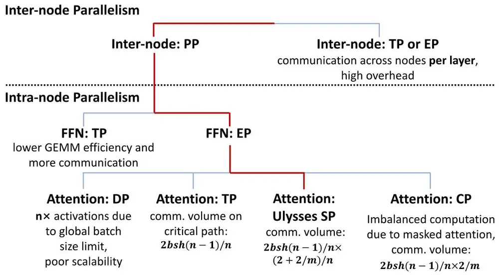
Tree diagram: inter-node PP versus inter-node TP or EP, then intra-node FFN TP or EP, then attention DP, TP, Ulysses SP or CP with their communication volumes; a red path selects PP, EP and Ulysses SP. — Figure 4 of the paper (a design diagram). The red path is the chosen layout: PP across nodes, EP for the FFN and Ulysses SP for attention inside the node. Each attention option shows its communication volume.論文圖 4（設計示意圖）。紅色路徑是選定的配置：跨節點用 PP，節點內 FFN 用 EP、注意力用 Ulysses SP。每個注意力選項都標出它的通訊量。Jin et al., EuroSys 2026, Figure 4 (arXiv 2505.11432v3 HTML, vector figure).

Diagram A shows what crosses which link. NVLink carries SP and EP traffic in every layer. The NICs carry PP activations and, once per step, DP gradients and parameters. DeepEP sends tokens to up to 4 nodes because cross-node bandwidth is low, and the paper notes that this restricts routing (§8). Here a token may pick any top- $k$ experts, because all of them are in the node.

示意圖 A 呈現哪些流量走哪條鏈路。NVLink 承載每一層的 SP 與 EP 流量。NIC 承載 PP 激活值，以及每一步一次的 DP 梯度與參數。DeepEP 因為跨節點頻寬低，只把 token 送到最多 4 個節點，論文指出這限制了路由（§8）。在這裡，token 可以選任何 top- $k$ 專家，因為它們全都在節點內。

Diagram A. Traffic per link in the evaluated layout (PP = 15, 8 GPUs per stage; blue squares are GPUs). Only PP (orange arrows) and DP (amber arrows) cross the NICs, which the paper does not describe.示意圖 A。評估配置中各鏈路的流量（PP = 15，每段 8 顆 GPU；藍色方塊是 GPU）。只有 PP（橘色箭頭）與 DP（琥珀色箭頭）經過 NIC，而論文沒有描述 NIC。Drawn for this primer from Jin et al., EuroSys 2026, §3, §6 and Figure 4.

The price is that EP cannot be larger than the node. The 32-expert 352B model holds 4 experts per GPU.

代價是 EP 不能比節點大。有 32 個專家的 352B 模型，每顆 GPU 放 4 個專家。

3.2 Count the bytes: SP for attention, EP for the experts3.2 計算位元組：注意力用 SP，專家用 EP

Table 1 of the paper names the symbols: micro-batch $b$ , sequence length $s$ , hidden size $h$ , parallel size $n$ , the ratio $m$ of query heads to key-value heads, and top- $k$ . TP all-gathers the input of attention and reduce-scatters its output. Ulysses-style sequence parallelism (SP) instead uses an all-to-all to give each GPU all tokens of some heads. K and V have $1/m$ as many heads as Q, so they are cheap. Per GPU per layer, formulas (1) and (2) are

論文 Table 1 定義符號：micro-batch $b$ 、序列長度 $s$ 、隱藏維度 $h$ 、平行大小 $n$ 、查詢頭數與鍵值頭數之比 $m$ ，以及 top- $k$ 。TP 對注意力的輸入做 all-gather、對輸出做 reduce-scatter。Ulysses 式的序列平行（SP）則用 all-to-all，讓每顆 GPU 取得部分 head 的所有 token。K 與 V 的 head 數只有 Q 的 $1/m$ ，所以很便宜。每顆 GPU 每層的量，公式 (1) 與 (2) 為

V^{\text{attn}}_{\mathrm{TP}} = 2bsh\,\frac{n-1}{n}, \qquad V^{\text{attn}}_{\mathrm{SP}} = 2bsh\,\frac{n-1}{n}\cdot\frac{2+2/m}{n}

SP moves $(2+2/m)/n$ of TP's bytes: 0.31 at $n = 8$ and $m = 4$ , which the paper calls about one fourth. Context parallelism would move less, but under a causal mask the GPUs get unequal work. For the FFN, expert parallelism sends each token to $k$ experts, so its volume is $k/n$ of TP's (formulas 3 and 4):

SP 搬的位元組是 TP 的 $(2+2/m)/n$ ：在 $n = 8$ 、 $m = 4$ 時是 0.31，論文稱之為約四分之一。context parallelism 搬得更少，但在因果遮罩下各 GPU 的工作量不相等。對 FFN，專家平行把每個 token 送到 $k$ 個專家，所以通訊量是 TP 的 $k/n$ （公式 3 與 4）：

V^{\text{FFN}}_{\mathrm{EP}} = \frac{k}{n}\cdot 2bsh\,\frac{n-1}{n}, \qquad V^{\text{FFN}}_{\mathrm{TP}} = 2bsh\,\frac{n-1}{n}

For the 352B model of the evaluation, with one sequence per micro-batch ( $b = 1$ , our assumption) in BF16:

以評估中的 352B 模型為例，每個 micro-batch 一條序列（ $b = 1$ ，我們的假設），使用 BF16：

Question問題	Calculation算式	Result結果
Activations $bsh$ in BF16 (Table 2 shapes)激活值 $bsh$ ，BF16（Table 2 的形狀）	$8192 \times 4096 \times 2$	$\approx 67.1$ MB
TP attention, (1), $n = 8$ TP 注意力，(1)， $n = 8$	$2 \times 67.1 \times 7/8$	$\approx 117.4$ MB
SP attention, (2), $m = 4$ SP 注意力，(2)， $m = 4$	$117.4 \times (2 + 2/4)/8$	$\approx 36.7$ MB
EP all-to-all, (3), top-3EP all-to-all，(3)，top-3	$117.4 \times 3/8$	$\approx 44.0$ MB
Layer, TP + TP over SP + EP一層：TP + TP 對 SP + EP	$(117.4 + 117.4)/(36.7 + 44.0)$	$\approx 2.9\times$
Dispatch per token, $k \times h \times 2\,\text{B}$ 每個 token 的 dispatch， $k \times h \times 2\,\text{B}$	$3 \times 4096 \times 2$	24,576 B7/8 leaves the GPU7/8 離開本 GPU

When $k$ exceeds $n$ , an all-to-all would move more bytes than an all-gather of every token, so EP switches collective (Diagram B; Figure 6 of the paper).

當 $k$ 超過 $n$ 時，all-to-all 搬的位元組會比把每個 token 都 all-gather 還多，所以 EP 改用另一種集體通訊（示意圖 B；論文 Figure 6）。

Diagram B. The two EP paths of Figure 6 of the paper (orange: NVLink collectives, green: expert GEMMs, plain: local copies). The all-to-all moves

k/n

of the TP volume

V

; the all-gather path always moves

V

.示意圖 B。論文 Figure 6 的兩條 EP 路徑（橘色：NVLink 集體通訊，綠色：專家 GEMM，無底色：本地複製）。all-to-all 搬 TP 通訊量

V

的

k/n

；all-gather 路徑永遠搬

V

。Drawn for this primer from Jin et al., EuroSys 2026, §3.2, Eqs. 3–4 and Figures 6–7.

The switch comes before $k = n$ . All-to-all talks to every peer, while all-gather and reduce-scatter are rings of neighbours (§3.2). Figure 7 of the paper (below) measured the crossover at top-6.

切換點在 $k = n$ 之前。all-to-all 要與每個同伴通訊，而 all-gather 與 reduce-scatter 是鄰居組成的環（§3.2）。論文 Figure 7（下圖）量到的交叉點在 top-6。

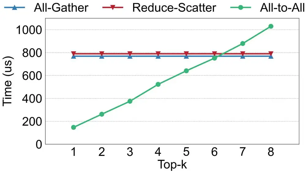
Line chart of time in microseconds versus top-k from 1 to 8: all-gather and reduce-scatter flat near 800, all-to-all rising from about 150 to about 1,030. — Figure 7 of the paper: dispatch collectives for Mixtral-8×7B versus top- $k$ (measured in one 8-GPU node). All-to-all grows from about 150 µs to about 1,030 µs (read from the plot); all-gather and reduce-scatter stay near 770–790 µs.論文圖 7：Mixtral-8×7B 的 dispatch 集體通訊對 top- $k$ （在一個 8 GPU 節點內量測）。all-to-all 從約 150 µs 增加到約 1,030 µs（由圖讀出）；all-gather 與 reduce-scatter 維持在約 770–790 µs。Jin et al., EuroSys 2026, Figure 7 (arXiv 2505.11432v3 HTML, vector figure).

At top-8 both paths move the same bytes, yet the all-to-all took about a third longer. Load balance uses an auxiliary loss and token dropping per GPU, as in DeepSeek-V2. The paper gives no skew data, and the skew stays on NVLink. The panel applies the formulas and the ratio $R$ of §3.4 to the models of Table 2.

在 top-8 時兩條路徑搬的位元組相同，all-to-all 卻多花了約三分之一的時間。負載平衡和 DeepSeek-V2 一樣，以每顆 GPU 為單位使用輔助損失與 token 丟棄。論文沒有提供偏斜資料，而偏斜留在 NVLink 上。面板把這些公式與 §3.4 的比值 $R$ 套到 Table 2 的模型上。

Panel 1面板 1

Bytes per MoE layer, and can the experts hide them?每個 MoE 層的位元組，以及專家計算能否遮住它們？

Model (Table 2)模型（Table 2）

Link for EP trafficEP 流量的鏈路

Model-parallel size

n

模型平行大小

n

Top-

k

Top-

k

Attention bytes

注意力位元組

FFN bytes (EP)

FFN 位元組（EP）

Dispatch collective

dispatch 集體通訊

Ratio

R

(§7 model)

比值

R

（§7 模型）

Dispatch per token

每個 token 的 dispatch

Our calculator of the paper's formulas (1)–(4) and of the ratio $R$ in §7, not the paper's code. Bytes are per GPU per MoE layer in the forward pass, for one sequence of 8,192 tokens ( $b = 1$ , our assumption) in BF16; model shapes come from Table 2. The all-to-all is taken to run at 75% of the all-gather's efficiency, the value at which the switch falls at top-6 for $n = 8$ , as Figure 7 measured. Compute assumes the H800 peak (989 TFLOP/s, Table 4). Link rates are taken at face value (NVLink 400 GB/s from Table 4, NIC 50 GB/s from Appendix A.1), so the times are lower bounds. Defaults: the 352B model, $n = 8$ , top-3, NVLink. Measured on this layout: SP + EP gave 1.13× the throughput of TP + TP on 240 H800 (Table 5). Try DS-MoE: its narrow experts give $R$ below 1 even on NVLink. Then pick the NIC: this is what EP across nodes would face. Raise $n$ : SP and EP bytes fall, TP bytes do not.

這是我們依論文公式 (1)–(4) 與 §7 比值 $R$ 所做的計算器，不是論文的程式碼。位元組是每顆 GPU 每個 MoE 層前向傳遞的量，對象是一條 8,192 token 的序列（ $b = 1$ ，我們的假設），使用 BF16；模型形狀取自 Table 2。我們假設 all-to-all 的效率是 all-gather 的 75%，這個值讓 $n = 8$ 時的切換點落在 top-6，與 Figure 7 的量測相符。計算以 H800 峰值為準（989 TFLOP/s，Table 4）。鏈路速率照標稱值計算（NVLink 400 GB/s 取自 Table 4，NIC 50 GB/s 取自附錄 A.1），所以時間是下限。預設值：352B 模型、 $n = 8$ 、top-3、NVLink。這個配置的實測：在 240 顆 H800 上，SP + EP 的吞吐量是 TP + TP 的 1.13 倍（Table 5）。試試 DS-MoE：它窄小的專家即使在 NVLink 上也讓 $R$ 低於 1。再選 NIC：這就是跨節點 EP 要面對的情況。把 $n$ 調大：SP 與 EP 的位元組下降，TP 的不會。

Stop and think

停下來想一想

Pick DS-MoE (narrow experts, top-6) and the NIC. Why must such a model keep its EP traffic on the scale-up network?

選 DS-MoE（窄小的專家，top-6）與 NIC。為什麼這樣的模型必須把 EP 流量留在 scale-up 網路上？

3.3 Hide what is left: two levels of overlap3.3 遮住剩下的：兩個層次的重疊

Inter-operator overlap. MegaScale-MoE writes the forward and backward pass of a whole MoE layer as explicit operators instead of torch.autograd. Communication runs on separate CUDA streams beside independent work. Selective activation rematerialization (SAR) recomputes or re-communicates cheap activations in the backward pass, hidden behind other work. Activation memory per layer falls from $(2n+2k+3kf+12+5/m)\,bsh/n$ to $(2kf+4+2/m)\,bsh/n$ , with $f$ the expert width over $h$ : about half.

運算子間重疊。MegaScale-MoE 把整個 MoE 層的前向與反向寫成明確的運算子，而不用 torch.autograd。通訊在獨立的 CUDA stream 上，與互不相依的工作並行。選擇性激活值重建（SAR）在反向傳遞中重新計算或重新通訊便宜的激活值，並藏在其他工作後面。每層激活值記憶體從 $(2n+2k+3kf+12+5/m)\,bsh/n$ 降到 $(2kf+4+2/m)\,bsh/n$ ，其中 $f$ 是專家寬度與 $h$ 之比：約減半。

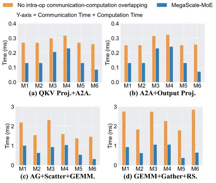
Intra-operator overlap. Forward dispatch has nothing independent to hide behind without a second micro-batch. So MegaScale-MoE fuses each collective into its GEMM and splits both into tiles (Diagram C). Device-memory flags signal each tile, without the host. Copy engines or a few tuned SMs move the data, and tile swizzling avoids NVLink contention.

運算子內重疊。沒有第二個 micro-batch 時，前向 dispatch 沒有可以躲在後面的獨立工作。所以 MegaScale-MoE 把每個集體通訊融合進它的 GEMM，並把兩者切成 tile（示意圖 C）。裝置記憶體中的旗標為每個 tile 發出訊號，不經主機。資料由 copy engine 或少數調校過的 SM 搬運，tile swizzling 則避免 NVLink 競爭。

Diagram C. The AG + scatter + GroupedGEMM kernel of §4.2. (a) The GEMM waits for the whole all-gather. (b) Each tile starts when its tokens arrive.示意圖 C。§4.2 的 AG + scatter + GroupedGEMM kernel。(a) GEMM 要等整個 all-gather 完成。(b) 每個 tile 在它的 token 到達時就開始。Drawn for this primer from Jin et al., EuroSys 2026, §4.2 and Figure 10.

A GroupedGEMM runs the matrix products of several experts in one kernel. Tokens are sorted by expert, then by source rank, so each tile waits on few ranks.

GroupedGEMM 在一個 kernel 中執行多個專家的矩陣乘法。token 先依專家、再依來源 rank 排序，讓每個 tile 只等少數幾個 rank。

3.4 Make each byte smaller, and the ratio that decides3.4 讓每個位元組變小，以及決定成敗的比值

Compression targets the NIC traffic. Gradients accumulate in FP32 and are cast to BF16 once. An all-to-all gives each GPU its shard from every DP peer, and the GPU sums the shards in FP32. A BF16 ring reduce-scatter would add in BF16 at every hop. Gradient bytes fall by 50%. In FP8 training with TP, the forward reduce-scatter becomes an FP8 all-to-all summed in FP32, with per-token scales. A four-step hierarchical scheme keeps SP's inter-node parameter bytes equal to TP's (Appendix A.1).

壓縮針對 NIC 上的流量。梯度以 FP32 累加，再一次轉成 BF16。all-to-all 讓每顆 GPU 從每個 DP 同伴取得自己那一份，再以 FP32 相加。環狀的 BF16 reduce-scatter 會在每一跳以 BF16 相加。梯度位元組減少 50%。在使用 TP 的 FP8 訓練中，前向 reduce-scatter 改成以 FP32 加總的 FP8 all-to-all，並以每個 token 為單位縮放。四步驟的階層方案讓 SP 的跨節點參數位元組與 TP 相同（附錄 A.1）。

§7 models whether EP survives a slower link, with expert width $h_{\text{ff}}$ , bandwidth $B$ and peak compute $P$ :

§7 用模型檢查 EP 在較慢的鏈路上是否仍可行，其中 $h_{\text{ff}}$ 是專家寬度、 $B$ 是頻寬、 $P$ 是峰值算力：

R = \frac{T_{\text{comp}}}{T_{\text{comm}}} = \frac{3}{2}\, h_{\text{ff}}\, \frac{B}{P}\cdot\frac{n}{n-1} \approx \frac{3}{2}\, h_{\text{ff}}\, \frac{B}{P}

Overlap hides EP only if $R > 1$ . $R$ does not depend on the number of experts, top- $k$ or $n$ . With the H800 numbers, our arithmetic gives $R \approx 9.9$ for the 352B experts on NVLink, $R \approx 1.2$ over a 50 GB/s NIC, and $R \approx 0.98$ for DeepSeekMoE on NVLink. These are model values.

只有 $R > 1$ 時，重疊才能遮住 EP。 $R$ 與專家數、top- $k$ 或 $n$ 無關。用 H800 的數字，我們算出 352B 的專家在 NVLink 上 $R \approx 9.9$ ，經 50 GB/s NIC 時 $R \approx 1.2$ ，DeepSeekMoE 在 NVLink 上 $R \approx 0.98$ 。這些是模型值。

4. Implementation4. 實作

The paper calls MegaScale-MoE ByteDance's production system. It runs most of the company's large MoE training, with single jobs on more than 10,000 GPUs for months (§7). One job trains a 200B model with 20B active parameters (Figure 20). The paper gives no lines of code and no kernel libraries; operator order and SM counts are tuned by hand.

論文稱 MegaScale-MoE 是字節跳動的生產系統。它執行公司大部分的大型 MoE 訓練，單一工作曾在超過 10,000 顆 GPU 上執行數個月（§7）。其中一個工作訓練一個啟用 20B 參數的 200B 模型（Figure 20）。論文沒有給出程式碼行數或 kernel 函式庫；運算子順序與 SM 數都由人工調校。

5. What was measured5. 量到了什麼

Setup. H800 GPUs (989 TFLOP/s, NVLink 400 GB/s; Table 4), 8 per node. The baseline is Megatron-LM with TP = 8 in the node. Both systems use PP = 15, sequence length 8,192 and the same batch. The NICs and the fabric are not described. Strong scaling (Table 3, 352B model, batch 720 sequences):

設定。H800 GPU（989 TFLOP/s、NVLink 400 GB/s；Table 4），每個節點 8 顆。基準是節點內 TP = 8 的 Megatron-LM。兩個系統都用 PP = 15、序列長度 8,192 與相同的批次。論文沒有描述 NIC 與網路。強擴展（Table 3，352B 模型，批次 720 條序列）：

GPUsGPU 數	Megatron-LM tokens/s	MegaScale-MoE tokens/s	Speedup加速	Days for 1T tokens1T token 天數
240	151.1k	272.9k	1.81×	42.41 / 76.61
480	301.1k	498.6k	1.65×	23.21 / 38.38
720	430.5k	740.1k	1.72×	15.64 / 26.88
960	550.2k	963.8k	1.77×	12.01 / 21.23
1,440	746.6k	1,407.7k	1.88×	8.22 / 15.50

Days are MegaScale-MoE / Megatron-LM. MFU fell from 32.48% to 27.89%, and the paper blames fewer micro-batches per pipeline. Its own numbers agree:

天數為 MegaScale-MoE / Megatron-LM。MFU 從 32.48% 降到 27.89%，論文歸因於每條管線的 micro-batch 變少。它自己的數字也吻合：

Question問題	Calculation算式	Result結果
DP replicas at 240 / 1,440 GPUs (120 GPUs each)240 / 1,440 顆 GPU 的 DP 副本數（每個 120 顆）	$240/120,\ 1440/120$	2 and 12
Sequences per replica per step每個副本每步的序列數	$720/2,\ 720/12$	360 and 60
Throughput at 1,440 GPUs (4.19 s per step)1,440 顆 GPU 的吞吐量（每步 4.19 s）	$720 \times 8192 / 4.19$	$\approx 1.41$ M tokens/s
Per-GPU throughput kept, against the MFU ratio每顆 GPU 保留的吞吐量，對照 MFU 比值	$\dfrac{1{,}407{,}700/1440}{272{,}900/240},\ \dfrac{27.89}{32.48}$	$\approx 0.86$ and $0.86$

So pipeline bubbles explain the drop. The paper shows no network profile that would rule out the network.

所以管線空泡解釋了這個下降。論文沒有提供能排除網路因素的網路剖析。

Weak scaling (Figure 12, 480–1,440 GPUs) gave 1.74–1.79×, and per-GPU throughput fell 0.2% against 2.74% for Megatron-LM. Ablation (Table 5, 240 GPUs): SP + EP gives 1.13×, inter-operator overlap 1.22× and intra-operator overlap 1.28×. On one node, SP + EP beat TP + TP by 14.9–32.9% in MFU at 1.2–5.4% more memory (Figure 14). SP and TP parameter synchronization differed by 0.3–3.1% (Figure 15). The fused kernels cut each operator pair's time by 1.2–4.7× and the iteration time by 7.1–12.9% (Figure 16, below).

弱擴展（Figure 12，480–1,440 顆 GPU）得到 1.74–1.79 倍，每顆 GPU 吞吐量下降 0.2%，Megatron-LM 則下降 2.74%。消融（Table 5，240 顆 GPU）：SP + EP 得到 1.13 倍，加上運算子間重疊為 1.22 倍，再加運算子內重疊為 1.28 倍。在單一節點上，SP + EP 的 MFU 比 TP + TP 高 14.9–32.9%，記憶體多 1.2–5.4%（Figure 14）。SP 與 TP 的參數同步只差 0.3–3.1%（Figure 15）。融合 kernel 讓每組運算子的時間縮短 1.2–4.7 倍，迭代時間減少 7.1–12.9%（下方 Figure 16）。

Four bar charts for models M1 to M6: orange bars without overlap are about 2 to 3 times taller than blue bars with fused kernels; FFN charts reach 3 ms, attention charts 0.4 ms. — Figure 16 of the paper (re-arranged into two rows): time of each operator pair without (orange) and with (blue) the fused kernels, for the models M1–M6 of Table 2, measured on H800 GPUs. The FFN pairs (c, d) gain most.論文圖 16（重排成兩列）：各運算子組合在沒有（橘色）與使用（藍色）融合 kernel 時的時間，涵蓋 Table 2 的模型 M1–M6，在 H800 GPU 上量測。FFN 的組合（c、d）增益最大。Jin et al., EuroSys 2026, Figure 16 (arXiv 2505.11432v3 HTML, vector figure; layout changed for phones).

SAR cut activation memory by 45.5–57.2% with MFU within 0.5% (Figure 17). The BF16 gradient all-to-all (7B MoE) and FP8 (35B and 176B models) gave loss curves that match their baselines (Figures 18–19); the paper gives no loss gaps.

SAR 讓激活值記憶體減少 45.5–57.2%，MFU 差距在 0.5% 以內（Figure 17）。BF16 梯度 all-to-all（7B MoE）與 FP8（35B 與 176B 模型）的損失曲線都與基準相符（Figures 18–19）；論文沒有給出損失差距。

6. Limits and open questions6. 限制與未解的問題

The network is out of view: no NIC count, link rate, topology, transport or profile of inter-node traffic.網路不在視野內：沒有 NIC 數、鏈路速率、拓樸、傳輸協定，也沒有跨節點流量的剖析。
The node caps EP. §7 leaves open whether SP and EP work at RDMA bandwidth. By $R$ , wide experts would and narrow ones would not; this is a model.節點限制了 EP。§7 沒有回答 SP 與 EP 在 RDMA 頻寬下是否可行。依 $R$ ，寬的專家可以，窄的不行；這是模型推論。
One baseline: Megatron-LM with TP = 8. There is no measured comparison with DeepEP or DualPipe.只有一個基準：TP = 8 的 Megatron-LM。沒有與 DeepEP 或 DualPipe 的實測比較。
MFU is 27.89% at 1,440 GPUs. The paper blames small GroupedGEMMs, dynamic shapes and CPU jitter in kernel launches.MFU 為 27.89%（1,440 顆 GPU）。論文歸因於小型 GroupedGEMM、動態形狀，以及 kernel 啟動時的 CPU 抖動。

7. How it connects7. 與其他內容的關聯

Deep dive, sections 3 and 5: the same TP and EP byte formulas; this paper keeps both on NVLink. In the Chapter 4, section 9.4, all-to-all skew hurts the network; here it never reaches the NICs.第 3 章第 3 與第 5 節：相同的 TP 與 EP 位元組公式；本論文把兩者都留在 NVLink 上。第 4 章第 9.4 節中，all-to-all 的偏斜會傷害網路；在這裡它從不碰到 NIC。
MegaScale is the same company's system for dense models. Rail-only measured an 8.2–11.2% cost when EP crosses rails; EP in the node avoids it.MegaScale 是同一家公司訓練稠密模型的系統。Rail-only 量到 EP 跨 rail 有 8.2–11.2% 的代價；EP 留在節點內就避開了。
MixNet makes the opposite bet and re-wires optics for cross-node EP; Odin controls congestion when the all-to-all reaches the network.MixNet 押相反的注，為跨節點 EP 重新接光纖；Odin 在 all-to-all 上了網路時控制壅塞。
EPIC removes duplicate inter-host EP bytes; UBEP works in a 384-NPU superpod, which would lift the node cap. HPN keeps an any-to-any tier for such traffic.EPIC 去除重複的跨主機 EP 位元組；UBEP 在 384 顆 NPU 的 superpod 中運作，可解除節點的上限。HPN 為這類流量保留 any-to-any 的一層。

Key numbers關鍵數字

Number	數字	Meaning (measured on H800 unless noted)
43.6% / 32%	Communication share of forward / training time (Hopper, setup not stated)	通訊占前向 / 訓練時間的比例（Hopper，設定未說明）
1,407.7k vs 746.6k	Tokens/s, 352B model on 1,440 GPUs, vs Megatron-LM	352B 模型在 1,440 顆 GPU 上的 tokens/s，對 Megatron-LM
32.48% → 27.89%	MFU, 240 → 1,440 GPUs	MFU，240 → 1,440 顆 GPU
1.13 / 1.22 / 1.28×	SP + EP, then the two overlaps (Table 5)	SP + EP，再加兩種重疊（Table 5）
7.1–12.9%	Iteration time saved by fused kernels	融合 kernel 省下的迭代時間
top- $k$ > 6	All-gather dispatch beats all-to-all (Mixtral-8×7B)	all-gather dispatch 勝過 all-to-all（Mixtral-8×7B）
> 10,000 GPUs	Production jobs, months long (§7)	生產環境工作，長達數月（§7）

Terms used on this page本頁用到的術語

Expert / top- $k$: One FFN of an MoE layer; a router sends each token to its $k$ best experts.; MoE 層中的一個 FFN；路由器把每個 token 送到它最合適的 $k$ 個專家。
EP: Expert parallelism: different experts on different GPUs.; 專家平行：不同的專家放在不同的 GPU 上。
SP (Ulysses): Sequence parallelism: an all-to-all gives each GPU all tokens of some attention heads.; 序列平行：all-to-all 讓每顆 GPU 取得部分注意力 head 的所有 token。
GroupedGEMM: One kernel for the matrix products of several experts.; 用一個 kernel 執行多個專家的矩陣乘法。
SAR: Selective activation rematerialization: recompute cheap activations instead of storing them.; 選擇性激活值重建：重新計算便宜的激活值，而不是存起來。
MFU: Model FLOPs utilization: useful FLOPs per second over peak.; 模型 FLOPs 使用率：每秒有用的 FLOPs 除以峰值。