Research digest 3 of 16 · Chapter 4: Collective communication

研究導讀 3 / 16 · 第 4 章：集體通訊

OptCCL: Scalable Synthesis of Optimal Collective Communication AlgorithmsOptCCL：可擴展地合成最佳集體通訊演算法

SIGCOMM 2026Richard Shapley, Rachit Agarwal, David Shmoys (Cornell University) · paper論文

After reading, you can explain why step-based schedule solvers trade optimality for scale, and how OptCCL routes first, schedules second and solves one subproblem per class of identical GPUs.讀完後，你能說明以時間步建模的排程求解器為何只能在最佳性與規模之間二選一，以及 OptCCL 如何先決定路由、再排程，並對每一類相同的 GPU 只解一個子問題。

≈ 11 min · 1 interactive panel · 5-question quiz≈ 11 分鐘 · 1 個互動面板 · 5 題測驗Chapter 4 ↗第 4 章 ↗Jump to the quiz ↓跳到測驗 ↓

If you read nothing else

只讀這一段也可以

Schedule synthesizers such as TE-CCL and SyCCL cut time into steps. Step size and step count are tied, so they get optimality or speed, not both: in most of the authors' runs they found no schedule beyond 16–64 GPUs within 3 hours. OptCCL solves space before time. A linear program (LP) picks the routes under bandwidth limits that hold only on average; the paper's Theorem 2 states that this loses nothing. Weighted fair queueing cuts the routes into fixed-size chunks, and a symmetry-aware decomposition solves one subproblem per class of identical GPUs. Measured synthesis time: hundreds of GPUs in tens of minutes, and 3–32× faster than SyCCL at 64 GPUs and more. The quality of the schedules was only simulated.

TE-CCL、SyCCL 這類排程合成器把時間切成步。步長與步數綁在一起，所以最佳性與速度只能擇一：在作者的大多數實驗中，它們在 3 小時內找不到超過 16–64 顆 GPU 的排程。OptCCL 先解空間、後解時間。一個線性規劃（LP）在只需平均成立的頻寬限制下選擇路由；論文的定理 2 指出這樣不損失任何東西。加權公平佇列（weighted fair queueing）把路由切成固定大小的 chunk，感知對稱性的分解法則對每一類相同的 GPU 只解一個子問題。實測的合成時間：數百顆 GPU 在數十分鐘內完成；在 64 顆 GPU 以上比 SyCCL 快 3–32 倍。排程本身的品質只做了模擬。

1. Where this paper sits1. 這篇論文的位置

Section 9.1 of the Chapter 4 asks whether a solver can beat ring and tree and still finish in time. TE-CCL solves multi-commodity flow on a time-expanded network, one copy of the network per time step: optimal, but it grows with GPUs, steps and chunks. SyCCL solves small sub-demands once and reuses them for isomorphic GPU groups: fast, but with no optimality guarantee. OptCCL (Cornell) claims every property of the paper's Table 1, part of which is below (★: possible with natural extensions).

第 4 章第 9.1 節問的是：求解器能否勝過環與樹，而且來得及算完。TE-CCL 在時間展開網路（time-expanded network）上解多商品流，每個時間步複製一份網路：它是最佳的，但規模隨 GPU、步數與 chunk 數成長。SyCCL 對小的子需求只解一次，再套用到同構的 GPU 群組：很快，但不保證最佳。OptCCL（Cornell）宣稱具備論文 Table 1 的所有性質，下表列出其中一部分（★：經自然延伸即可具備）。

System系統	Optimal最佳	Scalable可擴展	All collectives所有集體操作	Any hardware任意硬體	Concurrent collectives並行集體操作
NCCL	✗	✓	✓	✓	✓
TACCL	✗	✓	✓	✗	✗
SyCCL	✗	✓	✓	✗	✗
TE-CCL	✓	✗	✓	★	★
ForestColl	✓	✓	✗	✗	✗
OptCCL	✓	✓	✓	✓	✓

2. The problem: steps tie optimality to size2. 問題：時間步把最佳性與規模綁在一起

This argument is analysis, not measurement. A formulation with $T$ steps of size $s$ completes in $s \times T$ . The time-expanded network has one layer per step, so the LP grows roughly linearly with $T$ : we want few steps. But data enter a path one step at a time, so coarse steps leave links idle, a loss that grows with $s$ : we want small steps (Figure 1). With $s \times T$ fixed, we cannot have both. The exact integer program must also be solved for many candidate $s$ and $T$ , up to $|E| \times \log(|V| \times \text{data}/\text{chunk})$ times.

這個論點是分析，不是量測。一個有 $T$ 步、每步長 $s$ 的模型，完成時間是 $s \times T$ 。時間展開網路每一步一層，所以 LP 大約隨 $T$ 線性成長：我們希望步數少。但資料是一步一步進入路徑的，步長粗時鏈路會閒置，損失隨 $s$ 成長：我們希望步長小（圖 1）。 $s \times T$ 固定時，兩者無法兼得。精確的整數規劃還得對許多候選的 $s$ 與 $T$ 求解，最多 $|E| \times \log(|V| \times \text{資料量}/\text{chunk})$ 次。

Figure 1. The tussle on a three-link path. With 4 steps the collective ends at 2R, while with 16 it ends near R at the price of an LP with 4× the layers, and LP(9) has no steps at all. The step counts 4 and 16 show the trend that the paper describes.圖 1。三段鏈路路徑上的兩難。4 步時集體操作在 2R 才結束；16 步時接近 R，但 LP 的層數是 4 倍；LP(9) 沒有時間步。4 與 16 這兩個步數呈現論文所描述的趨勢。Drawn for this primer from Shapley et al., SIGCOMM 2026, §3.

Steps tie the spatial problem (which paths) to the temporal one (what crosses each link in each step). The evaluation measured where this stops: with each baseline's public code and a 3-hour limit, TE-CCL found no schedule beyond 16–32 GPUs, SyCCL none beyond 64–128, and TACCL scaled like SyCCL (§7.1).

時間步把空間問題（走哪些路徑）和時間問題（每一步每條鏈路傳什麼）綁在一起。評估量測了它在哪裡停下：使用各基準的公開程式碼、限時 3 小時，TE-CCL 超過 16–32 顆 GPU 就找不到排程，SyCCL 超過 64–128 顆也找不到，TACCL 與 SyCCL 相近（§7.1）。

3. The design: space first, then time3. 設計：先空間，後時間

OptCCL splits the problem into routing and scheduling (Figure 2).

OptCCL 把問題拆成路由與排程兩半（圖 2）。

Figure 2. OptCCL's pipeline. ① solves only the routing; ② checks every edge and, on a failure, splits a vertex and returns to ①; ③ emulates the routing with fixed-size chunks.圖 2。OptCCL 的流程。① 只解路由；② 逐邊檢查，不通過時拆分一個頂點並回到 ①；③ 用固定大小的 chunk 模擬這個路由。Drawn for this primer from Shapley et al., SIGCOMM 2026, §4.

3.1 The model and the usage variable3.1 模型與用量變數

Each component (GPU, CPU, memory, switch) can store, transmit, copy or reduce data, in any subset. The topology becomes a directed graph $G$ : an edge per link direction, a self-loop where data can be stored, and a shared limit $b(L)$ for each set $L$ of edges, such as a link or a memory. $G^T$ copies every vertex $T+1$ times (Figure 3).

每個元件（GPU、CPU、記憶體、交換器）可以儲存、傳送、複製或歸約資料，能力為任意子集。拓樸變成有向圖 $G$ ：每條鏈路的每個方向一條邊，能儲存資料之處有自迴圈，每組邊 $L$ （例如一條鏈路或一個記憶體）共用一個上限 $b(L)$ 。 $G^T$ 把每個頂點複製 $T+1$ 份（圖 3）。

Figure 1 of the OptCCL paper: a topology of 4 GPUs in two hosts with NICs and two rail switches, its directed graph with self-loops, and the time-expanded network — Figure 3. Figure 1 of the paper: 4 GPUs in two hosts with two rail switches (top left), OptCCL's graph with store loops (bottom left), and the time-expanded network, one layer per column (right). A design figure.圖 3。論文的 Figure 1：兩台主機中的 4 顆 GPU 與兩台 rail 交換器（左上）；OptCCL 的圖與儲存迴圈（左下）；時間展開網路，每一欄一層（右）。這是設計圖。Screenshot of Shapley et al., SIGCOMM 2026, Figure 1 (p. 3).

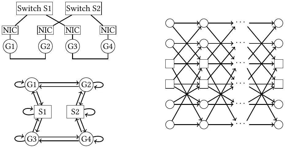
The objective is completion time; among optimal algorithms, OptCCL also minimizes a weighted sum of link bytes. A commodity is one sender–destination pair $(o,d)$ , with ordinary flow conservation for its flow $f_{e,o,d}$ . TE-CCL builds the collective's structure into its flow constraints; OptCCL adds a usage variable $w_{e,o}$ , the data of origin $o$ that edge $e$ really carries. One AllGather transmission can serve every destination, so:

目標是完成時間；在所有最佳演算法中，OptCCL 還最小化各鏈路位元組的加權和。一個商品（commodity）是一對發送端–目的端 $(o,d)$ ，其流 $f_{e,o,d}$ 遵守一般的流守恆。TE-CCL 把集體操作的結構寫進流量限制；OptCCL 則加上用量變數（usage variable） $w_{e,o}$ ，表示邊 $e$ 實際承載、來自起點 $o$ 的資料。AllGather 的一次傳送就能服務每個目的端，所以：

w_{e,o} \ge f_{e,o,d} \qquad \forall\, e,\ o,\ d

Usage covers the largest flow, not the sum: this is copy, written as a linear constraint.

用量只需涵蓋最大的流而非總和：這就是把複製寫成線性限制。

3.2 Route first: an LP over average bandwidth3.2 先路由：以平均頻寬寫成的 LP

OptCCL drops the per-step limit. It asks only that each edge set carry at most $R$ times its bandwidth over the target completion time $R$ :

OptCCL 拿掉每一步的上限，只要求每組邊在目標完成時間 $R$ 內承載的量不超過 $R$ 乘以其頻寬：

\sum_{t=0}^{T-1} \sum_{e \in L} \sum_{o} w_{\kappa(e,t),\,o} \;\le\; R\, b(L) \qquad \forall L

$\kappa(e,t)$ is edge $e$ in layer $t$ , and $T$ is now only a hop budget. Theorem 2: LP(9) and the step-based LP(7) convert into each other at equal cost and, up to any small $\epsilon$ , equal completion time, so one LP covers every step size. Max-flow problems give the optimal $R$ directly (a ForestColl technique).

$\kappa(e,t)$ 是第 $t$ 層的邊 $e$ ，此時 $T$ 只是跳數預算。定理 2：LP(9) 與時間步的 LP(7) 能以相同成本互相轉換，完成時間也只差任意小的 $\epsilon$ ，所以一個 LP 就涵蓋所有步長。最佳的 $R$ 由最大流問題直接算出（取自 ForestColl 的技巧）。

The LP can still cheat: the usage constraint assumes that flows from one origin on one edge carry the same data. OptCCL turns the routing into trees per sender and checks every edge. If all fit, the routing is optimal, since a relaxation's optimum is a lower bound. If not, it splits the offending vertex per destination and solves again (Figure 4).

LP 仍可能「作弊」：用量限制假設同一起點在同一條邊上的流都帶相同資料。OptCCL 把路由轉成每個發送端的樹，逐邊檢查。全部通過時路由就是最佳的，因為鬆弛問題的最佳值是下界。不通過時，就把出問題的頂點依目的端拆分，再解一次（圖 4）。

Figure 4. Left: two flows from o carry different data and share edge e, but the LP charges e one unit, as if they were one piece to be copied later. Right: u is split into u₁ and u₂, so the pieces need two units.圖 4。左：來自 o 的兩個流帶不同資料並共用邊 e，但 LP 只對 e 計一單位，彷彿它們是同一份資料、之後再複製。右：u 被拆成 u₁ 與 u₂，兩份資料便需要兩單位。Drawn for this primer from Shapley et al., SIGCOMM 2026, §4.2 and Figure 2.

Theorem 3: no repair is needed in an ideal topology, where optimal paths cross at most four links and the limits and costs sit on switch–NIC links. NVLink hosts on one tier of rail switches qualify when all data take the shortest path: the NIC is the bottleneck, and such paths are GPU → NIC → switch → NIC → GPU.

定理 3：在理想拓樸（ideal topology）中完全不必修補；這種拓樸的最佳路徑最多經過四條鏈路，上限與成本都位於交換器–NIC 鏈路。單層 rail 交換器連接的 NVLink 主機，在所有資料都走最短路徑時就符合：NIC 是瓶頸，這種路徑是 GPU → NIC → 交換器 → NIC → GPU。

3.3 Schedule second: fixed-size chunks by fair queueing3.3 後排程：以公平佇列產生固定大小的 chunk

Libraries send fixed-size chunks. OptCCL groups each sender's paths into a few trees with volumes $x_\tau$ and emulates them with weighted fair queueing (Parekh and Gallager). Each tree releases chunks of size $C$ at a steady rate, and a shared edge first sends the chunk with the smallest virtual time: when its data would finish there in the LP solution. Theorem 4 bounds the completion time $R_C$ with chunks:

函式庫傳送固定大小的 chunk。OptCCL 把每個發送端的路徑組成少數幾棵樹，各有量 $x_\tau$ ，並以加權公平佇列（Parekh 與 Gallager）模擬它們。每棵樹以穩定速率釋出大小 $C$ 的 chunk，共用的邊先送虛擬時間（virtual time）最小的 chunk：也就是在 LP 解中它的資料在該邊傳完的時間。定理 4 給出切成 chunk 後完成時間 $R_C$ 的上界：

\begin{gathered} R_C \le R\,(1+\gamma)\Big(1+\gamma+\frac{C\,T}{x_{\min}}\Big) \\ \gamma=\sqrt{\frac{2\,C\,T}{R\,b_{\min}}} \end{gathered}

$x_{\min}$ is the smallest tree volume and $b_{\min}$ the smallest bandwidth. If both carry far more than $CT$ bytes during $R$ , $R_C$ is close to $R$ ; larger collectives and scale only help.

$x_{\min}$ 是最小的樹量， $b_{\min}$ 是最小的頻寬。若兩者在 $R$ 內傳的量都遠大於 $CT$ 位元組， $R_C$ 就接近 $R$ ；集體操作與規模越大只會更好。

3.4 Every collective, any hardware3.4 所有集體操作、任意硬體

Switches without multicast: OptCCL adds flow conservation on the usage there, and splits a vertex only in corner cases; splitting every such vertex up front can nearly square the graph.不支援 multicast 的交換器：OptCCL 在這些頂點對用量加上流守恆，只在少數情況拆分頂點；若事先拆分所有這類頂點，圖可能接近平方倍。
AllReduce: some optimal AllReduce reduces every piece before it copies it (Theorem 5), yet a plain ReduceScatter then AllGather can still lose, so OptCCL solves both phases in one LP.AllReduce：存在一種最佳 AllReduce，先把每份資料歸約完再複製（定理 5），但單純先 ReduceScatter 再 AllGather 仍可能吃虧，所以 OptCCL 在一個 LP 中同時解兩個階段。
Others: All-to-All needs no usage variables, ReduceScatter is AllGather reversed, and concurrent collectives share the average limits under one objective, the makespan (the time to finish all).其他：All-to-All 不需要用量變數，ReduceScatter 是反向的 AllGather，並行的集體操作則在同一個目標 makespan（全部完成所需的時間）下共用平均上限。

3.5 Symmetry: one subproblem per class of GPUs3.5 對稱性：每一類 GPU 一個子問題

LP(9) for an AllGather on $n$ GPUs has $\Omega(n^3)$ variables, but only the bandwidth limits link the origins, through the usage variables. Dantzig–Wolfe decomposition uses this: a master problem holds those limits, and each origin's subproblem proposes routings under the master's prices, so each iteration solves $n$ subproblems.

$n$ 顆 GPU 的 AllGather，LP(9) 有 $\Omega(n^3)$ 個變數，但只有頻寬上限透過用量變數把各起點連在一起。Dantzig–Wolfe 分解利用這一點：主問題保存這些上限，每個起點的子問題依主問題給的價格提出路由，所以每次迭代要解 $n$ 個子問題。

Mirrored Dantzig–Wolfe adds symmetry. Two GPUs are indistinguishable if the input without labels looks the same from both. Theorem 6: a symmetric input has a symmetric optimal solution. So OptCCL solves one subproblem per class (Figure 5), each roughly $n^2$ times smaller than the LP, in the paper's words. SyCCL instead repeats each route pattern in every isomorphic group, which, the authors state, no longer guarantees optimality (shown in their technical report).

Mirrored Dantzig–Wolfe 再加上對稱性。若去掉標籤後，從兩顆 GPU 看出去的輸入都一樣，它們就無法區分。定理 6：對稱的輸入有對稱的最佳解。所以 OptCCL 每一類只解一個子問題（圖 5），依論文的說法，每個子問題大約比整個 LP 小 $n^2$ 倍。SyCCL 則讓每個路由模式在每個同構群組中重複；作者指出這樣就不再保證最佳（在其技術報告中說明）。

Figure 5. LP(9): one block per origin, linked by bandwidth rows (left). Dantzig–Wolfe solves a subproblem per origin per iteration (middle); the mirrored version solves one per class and relabels it with

\pi

(right).圖 5。LP(9)：每個起點一個區塊，靠頻寬限制列連結（左）。Dantzig–Wolfe 每次迭代為每個起點解一個子問題（中）；mirrored 版本每一類只解一個，再以

\pi

重新標號（右）。Drawn for this primer from Shapley et al., SIGCOMM 2026, §6.

Panel 1 sets the LP's size beside the measured synthesis times.

面板 1 把 LP 的大小與實測的合成時間並列。

Panel 1面板 1

How big is the LP, and how long did synthesis take?LP 有多大？合成花了多久？

Collective集體操作

Topology拓樸

GPUs

n

GPU 數

n

Layers

T

G^T

G^T

的層數

T

Monolithic LP(9): variables

整體 LP(9)：變數

One subproblem: variables

單一子問題：變數

Constraint matrix, whole ÷ one subproblem

限制矩陣，整體 ÷ 單一子問題

Subproblems per iteration

每次迭代的子問題數

OptCCL, measured synthesis

OptCCL 實測合成時間

Baselines at this size

此規模下的基準

Left: our own count of LP(9)'s size, not the paper's. The graph follows the paper's Figure 1: a vertex per GPU and per rail switch (the NIC folded into the GPU–switch link), links inside a host between every GPU pair, every link in both directions, a store loop on every vertex, and $T$ layers; $T = 4$ covers a path with one hop inside each host, GPU → GPU → switch → GPU → GPU. AllGather has a flow per edge and sender–destination pair plus a usage per edge and sender; All-to-All has flows only. A Dantzig–Wolfe subproblem keeps one sender. The paper states $\Omega(n^3)$ variables and subproblems "roughly a factor of $n^2$ " smaller; by our count a subproblem has about $n$ times fewer variables and $n$ times fewer constraints, so its constraint matrix is about $n^2$ times smaller. Right: measured synthesis times on the authors' 32-core server, read from the paper's Figures 4 and 5 (about $\pm 10\%$ on the log scale); a line that ends means no schedule within the 3-hour limit. Defaults: AllGather on the A100 topology, 64 GPUs, $T = 4$ . Try 64 → 256 GPUs: the LP grows about 64×, and OptCCL's measured time goes from about 1 minute to about 30 minutes. Then raise $T$ : a step-based LP needs one layer per time step.

左：我們自己計算的 LP(9) 規模，不是論文的數字。圖依論文 Figure 1 建立：每顆 GPU 與每台 rail 交換器一個頂點（NIC 併入 GPU–交換器鏈路），主機內每對 GPU 之間都有鏈路，每條鏈路兩個方向，每個頂點一個儲存迴圈，共 $T$ 層； $T = 4$ 涵蓋兩端主機內各有一跳的路徑 GPU → GPU → 交換器 → GPU → GPU。AllGather 每條邊、每對發送端–目的端各有一個流變數，每條邊、每個發送端各有一個用量變數；All-to-All 只有流變數。一個 Dantzig–Wolfe 子問題只保留一個發送端。論文陳述變數為 $\Omega(n^3)$ ，子問題「大約小 $n^2$ 倍」；依我們的計算，子問題的變數與限制各少約 $n$ 倍，所以限制矩陣約小 $n^2$ 倍。右：作者 32 核心伺服器上實測的合成時間，讀自論文 Figure 4 與 5（對數座標上約 $\pm 10\%$ ）；線條中斷表示在 3 小時上限內沒有排程。預設：A100 拓樸上的 AllGather、64 顆 GPU、 $T = 4$ 。試試從 64 到 256 顆 GPU：LP 約變大 64 倍，OptCCL 的實測時間從約 1 分鐘變成約 30 分鐘。再提高 $T$ ：以時間步建模的 LP 每一步都要一層。

4. Implementation4. 實作

The code is public on GitHub; the paper gives no language, solver or line count. Synthesis time covers one representative schedule per symmetry class, not its expansion to every GPU. Switches could only store and transmit (no multicast or in-network reduction). OptCCL is not yet integrated with NCCL or RCCL.

程式碼公開在 GitHub；論文沒有說明語言、求解器或程式行數。合成時間只涵蓋每個對稱類一個代表性排程，不包含展開到每顆 GPU。交換器只能儲存與傳送（沒有 multicast 或網內歸約）。OptCCL 尚未整合進 NCCL 或 RCCL。

5. What was measured5. 量到了什麼

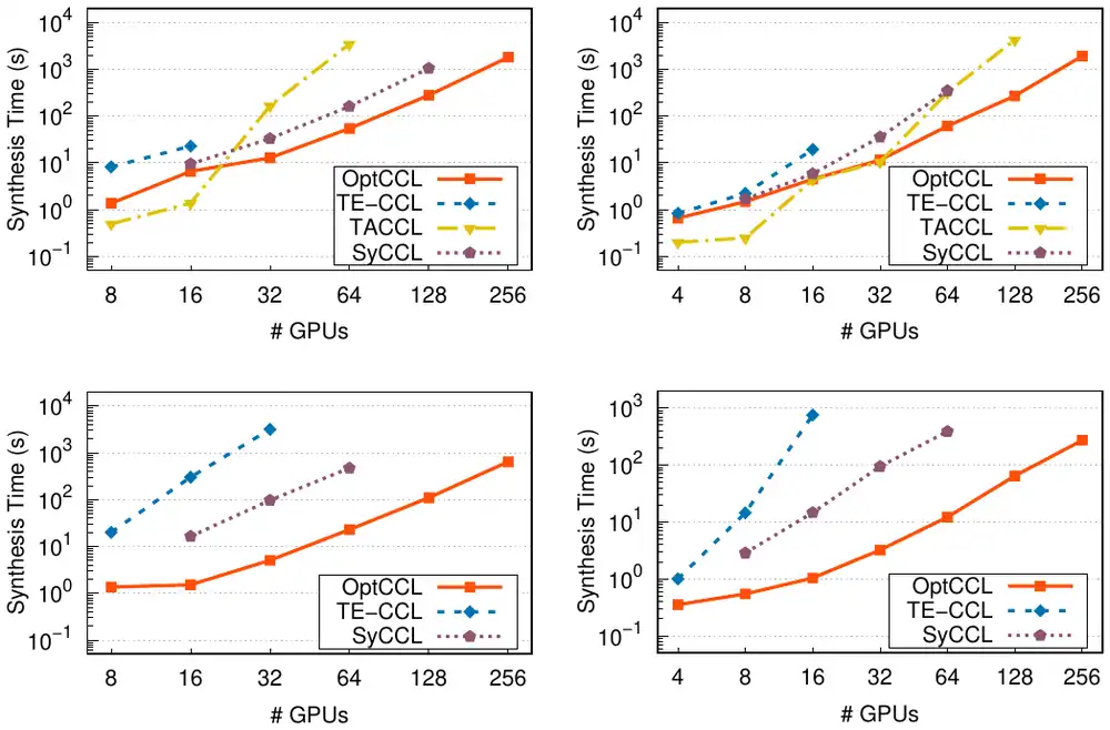
The topologies were "A100" (8 GPUs per host) and "DOE" (4 GPUs per host, after NERSC's Perlmutter), with NVLink inside hosts and a Rail-only-style multi-rail network between them, on 4 or 8 up to 256 GPUs. TE-CCL, SyCCL and TACCL ran from public code, each at the largest chunk count it finished within 3 hours; SyCCL cannot run one host, and TACCL's All-to-All has known bugs. Link bandwidths and data and chunk sizes are not stated.

拓樸是「A100」（每主機 8 顆 GPU）與「DOE」（每主機 4 顆 GPU，依 NERSC 的 Perlmutter），主機內為 NVLink，主機之間是 Rail-only 式的 multi-rail 網路，規模從 4 或 8 顆到 256 顆 GPU。TE-CCL、SyCCL 與 TACCL 以公開程式碼執行，各取 3 小時內能完成的最大 chunk 數；SyCCL 無法執行單一主機，TACCL 的 All-to-All 有已知錯誤。論文沒有說明鏈路頻寬、資料大小與 chunk 大小。

Only the synthesis times are measurements: the paper states that its evaluation uses simulations, so the bandwidth of every schedule and the concurrent-collective results are computed, not run, and this page leaves them out.

只有合成時間是量測值：論文說明其評估使用模擬，所以每個排程的頻寬與並行集體操作的結果都是計算而非實際執行，本頁略去不列。

Case情況	Measured synthesis time實測合成時間
Where the baselines stop (3 hours)基準停下的位置（3 小時）	TE-CCL beyond 16–32 GPUs, SyCCL beyond 64–128; TACCL like SyCCLTE-CCL 超過 16–32 顆 GPU、SyCCL 超過 64–128 顆；TACCL 與 SyCCL 相近
OptCCL, largest sizesOptCCL，最大規模	Hundreds of GPUs within tens of minutes; about 30 minutes for a 256-GPU AllGather (Figure 4)數百顆 GPU 在數十分鐘內；256 顆 GPU 的 AllGather 約 30 分鐘（Figure 4）
64 GPUs or more64 顆 GPU 以上	3–32× faster than SyCCL, 5–60× faster than TACCL比 SyCCL 快 3–32 倍，比 TACCL 快 5–60 倍
All-to-AllAll-to-All	2–500× faster than TE-CCL and SyCCL比 TE-CCL 與 SyCCL 快 2–500 倍
AllGather, 16 GPUs or fewerAllGather，16 顆 GPU 以下	TACCL often faster than OptCCL (Figure 4)TACCL 常比 OptCCL 快（Figure 4）

The paper credits much of the speed-up to Mirrored Dantzig–Wolfe, with details in its technical report. Figure 6 shows the measured curves.

論文把很大一部分的加速歸功於 Mirrored Dantzig–Wolfe，細節在其技術報告中。圖 6 是實測的曲線。

Synthesis-time panels of Figures 4 and 5 of the OptCCL paper: synthesis time in seconds on a log scale against the number of GPUs for OptCCL, TE-CCL, TACCL and SyCCL — Figure 6. Synthesis-time panels of the paper's Figures 4 and 5 (seconds, log scale): AllGather top, All-to-All bottom; A100 left, DOE right. A line that stops means no schedule within 3 hours (for SyCCL, also one host); TACCL has no All-to-All. Measured run times; the simulated bandwidth panels are left out.圖 6。論文 Figure 4 與 5 的合成時間子圖（秒，對數座標）：上為 AllGather，下為 All-to-All；左為 A100，右為 DOE。線條中斷表示 3 小時內沒有排程，SyCCL 則也可能是單一主機；TACCL 沒有 All-to-All。這些是實測的執行時間；模擬的頻寬子圖已略去。Screenshot of Shapley et al., SIGCOMM 2026, Figures 4 and 5, synthesis-time panels only (p. 11).

6. Limits and open questions6. 限制與未解的問題

The paper's own limits: a new collective needs carefully defined usage variables; the proofs and evaluation assume large messages, and small ones under the $\alpha$ – $\beta$ model are left for later; concurrent collectives optimize only the makespan; NCCL or RCCL integration and testbed validation come next. A careful reader adds:

論文自述的限制：新的集體操作需要仔細定義用量變數；證明與評估都假設大訊息， $\alpha$ – $\beta$ 模型下的小訊息留待之後；並行的集體操作只最佳化 makespan；下一步是整合進 NCCL 或 RCCL 並在測試平台驗證。細心的讀者還應補上：

Evidence and proofs. No schedule ran on hardware; the measured quantity is solver time on one server. Theorems 1–6 are proved in a technical report outside the reviewed paper.證據與證明。沒有任何排程在硬體上跑過；量到的是單一伺服器上的求解時間。定理 1–6 的證明在審稿論文之外的技術報告中。
Outside ideal topologies. A multi-tier Clos, or a host whose internal links bind, may need the split-and-solve loop, which in the worst case adds many vertices; the paper does not say how often its runs needed it.理想拓樸之外。多層 Clos，或主機內鏈路成為瓶頸時，可能需要「拆分再解」的迴圈，最壞情況會加入許多頂點；論文沒有說明實驗中多常用到它。
Static input. MoE sizes known only at run time, failed links and other tenants' traffic that is not given as input are outside the model.靜態輸入。執行時才知道的 MoE 大小、故障的鏈路與未列入輸入的其他租戶流量都在模型之外。
Baseline limits depend on settings. SyCCL's own paper reports about 37 minutes at 512 GPUs on its setup (the collectives research notes, 9.1).基準的上限取決於設定。SyCCL 自己的論文在其設定下回報 512 顆 GPU 約 37 分鐘（第 4 章第 9.1 節）。

7. How it connects7. 與其他內容的關聯

Deep dive, section 9.1: the third step after TE-CCL and SyCCL. It replaces TE-CCL's epochs with one average limit, and SyCCL's group symmetry with a symmetry that keeps optimality.第 4 章第 9.1 節：繼 TE-CCL 與 SyCCL 之後的第三步。它以一個平均上限取代 TE-CCL 的 epoch，以保持最佳性的對稱取代 SyCCL 的群組對稱。
Deep dive, section 4, and Rail-only: the paper's example of an ideal topology is the NVLink-plus-rail design, and the evaluation used Rail-only's network.第 4.4 節與 Rail-only：論文舉的理想拓樸例子正是 NVLink 加 rail 的設計，評估也使用 Rail-only 的網路。
MCCS, which OptCCL cites on why collective performance matters: a provider-run service sees the topology, so such a solver could run there.MCCS（OptCCL 引用它說明集體通訊效能的重要性）：供應商執行的服務看得到拓樸，這種求解器可以在那裡執行。
Theseus accepts new solver output while a job runs, so minutes of synthesis need not stop the job.Theseus 能在任務執行中接收求解器的新輸出，所以幾分鐘的合成不必讓任務停下。

Key numbers關鍵數字

Number	數字	Meaning (measured synthesis time unless noted)
16–32 / 64–128	GPUs beyond which TE-CCL / SyCCL found no schedule in 3 h	TE-CCL / SyCCL 超過此 GPU 數就在 3 小時內找不到排程
3–32× · 5–60×	OptCCL faster than SyCCL · TACCL, 64 GPUs or more	64 顆 GPU 以上，OptCCL 比 SyCCL · TACCL 快的倍數
2–500×	OptCCL faster than TE-CCL and SyCCL, All-to-All	All-to-All，OptCCL 比 TE-CCL 與 SyCCL 快的倍數
≈ 30 min	OptCCL, 256-GPU AllGather (Figure 4, read from the plot)	OptCCL，256 顆 GPU 的 AllGather（Figure 4，讀自圖）
$\Omega(n^3)$ · $\le 4$ links條鏈路	LP(9) variables for AllGather · path length of an ideal topology (analysis)	AllGather 的 LP(9) 變數 · 理想拓樸的路徑長度（分析）

Terms used on this page本頁用到的術語

Time-expanded network: $T+1$ copies of every vertex, with each edge joining one layer to the next.; 每個頂點複製 $T+1$ 份，每條邊把一層連到下一層。
Usage variable: The data of one origin that an edge really carries; at least the largest flow, not their sum.; 一條邊實際承載的、來自某個起點的資料；至少等於最大的流，而非總和。
Ideal topology: Optimal paths of at most four links, with limits on switch–NIC links; the LP alone is exact.; 最佳路徑最多四條鏈路，上限位於交換器–NIC 鏈路；光靠 LP 就是精確的。
Mirrored Dantzig–Wolfe: Dantzig–Wolfe decomposition with one subproblem per class of indistinguishable GPUs.; 對每一類無法區分的 GPU 只用一個子問題的 Dantzig–Wolfe 分解。