Research digest 2 of 2 · Chapter 1: What training computes

研究導讀 2 / 2 · 第 1 章：訓練在算什麼

Coflow Scheduling for LLM TrainingLLM 訓練的 coflow 排程

SIGCOMM 2025 (short paper)Xinchen Wan, Xinyu Yang, Kaiqiang Xu et al. (HKUST, USTC) · paper論文

After reading, you can explain what a coflow is, where the coflows of an MoE training job collide, and how Hermod's key (micro-batch, type, layer) decides which goes first.讀完後，你能說明什麼是 coflow、MoE 訓練任務的 coflow 在哪裡相撞，以及 Hermod 的鍵值（micro-batch、類型、層）如何決定誰先走。

≈ 10 min · 1 interactive panel · 5-question quiz≈ 10 分鐘 · 1 個互動面板 · 5 題測驗Chapter 1 ↗第 1 章 ↗Jump to the quiz ↓跳到測驗 ↓

If you read nothing else

只讀這一段也可以

A mixture-of-experts (MoE) training job sends three kinds of traffic between servers: expert-parallel (EP) all-to-all, pipeline-parallel (PP) sends, and data-parallel (DP) reduce-scatter and all-gather. Each communication step is a coflow, a group of flows that the next computation waits for as one unit. These coflows collide on links at predictable moments, and fair sharing serves them whether or not a GPU waits. Hermod, a short paper from HKUST, ranks every coflow of a job with one static key: micro-batch ID, then type (EP and PP before DP), then layer ID, lower first. The whole cluster applies the same order. The paper has no implementation and evaluates only in simulation, so this page teaches the mechanism and its reasoning and reports no speedups.

混合專家（MoE）訓練任務在伺服器之間送三種流量：專家平行（EP）的 all-to-all、管線平行（PP）的傳送，以及資料平行（DP）的 reduce-scatter 與 all-gather。每一個通訊步驟都是一個 coflow：一組流，下一段計算把它當成一個整體來等待。這些 coflow 會在可預測的時刻於鏈路上相撞，而公平分享不管有沒有 GPU 在等都一樣服務它們。Hermod 是香港科技大學的一篇短論文，它用一個靜態鍵值為任務的每個 coflow 排序：先比 micro-batch 編號，再比類型（EP 與 PP 先於 DP），最後比層編號，都是小的先。整個叢集都套用同一個順序。論文沒有實作，只在模擬中評估，所以本頁教的是機制與理由，不報告任何加速數字。

1. Where this paper sits1. 這篇論文的位置

Section 1.1, "The training step as a timeline", draws one GPU's step as rows: arithmetic, TP all-reduce, PP sends and DP reduce-scatter. Section 4 adds overlap: DP traffic hides behind the backward pass, and only the rest is exposed. Section 6 shows the result on the wire: a few large flows that start together.

第 1.1 節「把訓練步畫成時間線」把一顆 GPU 的一步畫成幾列：算術、TP all-reduce、PP 傳送與 DP reduce-scatter。第 4 節加入重疊：DP 流量藏在反向傳播後面，只有剩下的部分會暴露。第 6 節展示線上的結果：少數幾條同時開始的大流。

Chapter 1 treats each row alone. It does not ask which row should win when two want the same NIC. The question is sharpest for MoE models, whose all-to-all runs in every MoE layer of both passes (Chapter 3, section 5). Two end-host schedulers answered parts of it: ByteScheduler overlapped DP traffic layer by layer, and Lina put EP coflows ahead of DP coflows in the backward pass. Hermod's critique is that each covers only some coflow types, decides on one host, and ignores PP. Crux (SIGCOMM 2024) asks a different question: which job should win a shared link.

第 1 章把每一列分開處理。它沒有問：兩列同時要用同一張 NIC 時該讓哪一列先。這個問題在 MoE 模型上最尖銳，因為它的 all-to-all 在兩個方向的每個 MoE 層都會執行（第 3 章第 5 節）。兩個端主機排程器各回答了一部分：ByteScheduler 逐層重疊 DP 流量，Lina 在反向傳播中讓 EP coflow 先於 DP coflow。Hermod 的批評是：兩者都只涵蓋部分 coflow 類型、只在單一主機上決定，而且都忽略 PP。Crux（SIGCOMM 2024）問的是另一個問題：共用鏈路上該讓哪一個任務先走。

2. The problem, argued from the training graph2. 問題：從訓練圖推論出來

The paper has no measurement study; it argues from the structure of training. A coflow is the group of flows that serve one communication step, such as every flow of one all-to-all. The next computation waits for the last flow, so a coflow is done only when all its flows are. Hermod takes this model from Crux.

這篇論文沒有量測研究；它從訓練的結構來論證。coflow 是服務同一個通訊步驟的一組流，例如一次 all-to-all 的所有流。下一段計算等的是最後一條流，所以只有所有流都結束，coflow 才算完成。Hermod 的這個模型取自 Crux。

Congestion control shares a busy link roughly equally between flows, without knowing which one a GPU waits for. Take a 400 Gb/s link, which moves 50 MB per millisecond, and two coflows that start together: a 32 MB EP coflow that the next layer waits for, and a 128 MB DP coflow that nothing needs until the step ends. The sizes are ours; the paper gives none.

壅塞控制把忙碌的鏈路大致平均分給各條流，並不知道 GPU 在等哪一條。取一條 400 Gb/s 的鏈路，每毫秒搬 50 MB，以及兩個同時開始的 coflow：一個 32 MB 的 EP coflow，下一層在等它；一個 128 MB 的 DP coflow，在一步結束前沒有人需要它。大小是我們取的；論文沒有給任何大小。

Question問題	Calculation算式	Result結果
Fair share: EP gets half the link, 25 MB per ms公平分享：EP 分到半條鏈路，每 ms 25 MB	$32 \div 25$	$\approx 1.28$ ms
Fair share: DP has sent 32 MB by then; the rest at full rate公平分享：DP 這時已送 32 MB；其餘全速送出	$1.28 + (128 - 32) \div 50$	$\approx 3.2$ ms
EP first: EP alone on the linkEP 優先：EP 單獨使用鏈路	$32 \div 50$	$\approx 0.64$ ms
EP first: DP after itEP 優先：DP 接在後面	$0.64 + 128 \div 50$	$\approx 3.2$ ms

Priority halves the next layer's wait, and DP still ends at 3.2 ms: the link never idles, so its last byte leaves at the same moment (Figure A). Order decides who finishes first, not when the link finishes. Coflow schedulers for data-analytics clusters order coflows by size or by the bytes already sent. Hermod orders them by their position in the training graph.

優先權讓下一層的等待減半，而 DP 仍在 3.2 ms 結束：鏈路從不閒置，所以最後一個位元組在同一時刻離開（圖 A）。順序決定的是誰先完成，而不是鏈路何時完成。為資料分析叢集設計的 coflow 排程器依大小或已送出的位元組排序。Hermod 則依它們在訓練圖中的位置排序。

Figure A. Left: a coflow is done when its last flow is, and the GPU waits until then. Right: the example above on one link; bar height is the share of the link. Priority moves the end of the EP coflow from 1.28 to 0.64 ms, and DP ends at 3.2 ms either way.圖 A。左：coflow 在最後一條流結束時才完成，GPU 一直等到那時。右：上面的例子放在一條鏈路上；長條高度是占用鏈路的比例。優先權把 EP coflow 的結束時間從 1.28 ms 提前到 0.64 ms，而 DP 兩種情況都在 3.2 ms 結束。Drawn for this primer with example sizes.

The paper adds two gaps. Earlier training schedulers ignore PP, whose coflows form strict chains. And none handles imbalance inside one coflow, such as a skewed all-to-all; Hermod leaves that to future work.

論文還指出兩個缺口。先前的訓練排程器忽略 PP，而 PP 的 coflow 形成嚴格的先後鏈。而且沒有人處理單一 coflow 內部的不平衡，例如偏斜的 all-to-all；Hermod 把它留給未來的工作。

3. The design3. 設計

Hermod maps where coflows collide in the training graph, then gives a key that decides each collision.

Hermod 先標出 coflow 在訓練圖中相撞的地方，再給出一個決定每次相撞誰先走的鍵值。

3.1 The training graph and its coflows3.1 訓練圖與它的 coflow

Hermod schedules only traffic between servers: EP, PP and DP. Tensor parallelism stays inside a server. The topology, the parallelization strategy and the worker placement fix the training DAG (directed acyclic graph), so every coflow and every dependency is known before the first step.

Hermod 只排程伺服器之間的流量：EP、PP 與 DP。張量平行留在伺服器內。拓樸、平行化策略與 worker 配置固定了訓練 DAG（有向無環圖），所以每個 coflow 與每個依賴在第一步之前就已知道。

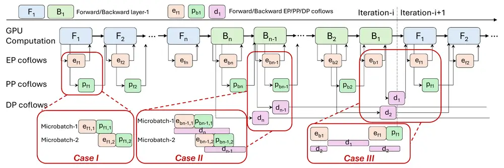
The paper's Figure 1 draws this DAG for one GPU that trains an MoE model with ZeRO-2 and 1F1B. ZeRO-2 shards gradients and optimizer state, so DP runs a reduce-scatter of gradients and an all-gather of parameters. 1F1B alternates the forward pass of a new micro-batch with the backward pass of an older one (Section 3.5). Every MoE layer group runs EP coflows, dispatch and gather; the paper says they occur twice per MoE layer group in each iteration, and its Figure 1 draws them in both passes, and a PP coflow carries the result onward. DP runs in the backward pass, and its all-gather continues into the next forward pass.

論文的圖 1 畫出一顆 GPU 以 ZeRO-2 與 1F1B 訓練 MoE 模型時的 DAG。ZeRO-2 把梯度與優化器狀態分片，所以 DP 對梯度做 reduce-scatter、對參數做 all-gather。1F1B 交替進行新 micro-batch 的前向與舊 micro-batch 的反向（第 1 章 03 第 4 節）。每個 MoE 層群組執行 EP coflow，分派與收回；論文說它們在每次迭代中每個 MoE 層群組出現兩次，而它的圖 1 在兩個方向都畫了它們，再由一個 PP coflow 把結果往下傳。DP 在反向期間執行，它的 all-gather 延續到下一次前向。

The paper's Figure 1: one GPU's computation row (forward F1 to Fn, backward Bn to B1, then the next iteration) above rows of EP, PP and DP coflows, with three red boxes marking overlap cases and enlarged views of Case I, Case II and Case III — The paper's Figure 1. Computation (forward F1…Fn, backward Bn…B1, then the next iteration) above the EP (e), PP (p) and DP (d) coflows; arrows are dependencies. Red boxes mark the three overlap cases, enlarged below. A schematic, not data.論文的圖 1。計算（前向 F1…Fn、反向 Bn…B1，然後是下一次迭代）位於 EP（e）、PP（p）與 DP（d）coflow 之上；箭頭是依賴。紅框標出三種重疊情況，並在下方放大。這是示意圖，不是資料。Wan et al., "Coflow Scheduling for LLM Training", ACM SIGCOMM 2025, Figure 1.

3.2 Three places where coflows collide3.2 coflow 相撞的三個地方

A pass over the DAG finds three cases of overlap, the red boxes:

走過一遍 DAG，會找到三種重疊情況，也就是那些紅框：

Case I. EP and PP coflows of two micro-batches overlap: micro-batch 1's are still on the wire when micro-batch 2 starts.情況 I。兩個 micro-batch 的 EP 與 PP coflow 重疊：micro-batch 2 開始時，micro-batch 1 的還在線上。
Case II. In the backward pass, EP and PP coflows of two micro-batches overlap the DP coflows of the last layers.情況 II。反向期間，兩個 micro-batch 的 EP 與 PP coflow 與最後幾層的 DP coflow 重疊。
Case III. At the iteration boundary, the next iteration's first EP and PP coflows overlap this iteration's DP of layers 1 and 2.情況 III。在迭代交界，下一次迭代最早的 EP 與 PP coflow 與本次迭代第 1、2 層的 DP 重疊。

In each case one fact of the DAG says which coflow blocks more work. Figure B shows the order that follows.

在每一種情況中，DAG 的某個事實說明了哪個 coflow 擋住更多工作。圖 B 畫出由此得到的順序。

Figure B. The three overlap cases. Top: the coflows that contend. Bottom: the order Hermod gives on one link; the arrow is time. e, p and d mark EP, PP and DP; the digit is the micro-batch (e, p) or the layer (d). e′ and p′ are the next iteration's layer-1 coflows; they must wait for d1 to deliver layer 1's parameters.圖 B。三種重疊情況。上：相互爭搶的 coflow。下：Hermod 在一條鏈路上給出的順序；箭頭是時間。e、p、d 分別代表 EP、PP、DP；數字是 micro-batch（e、p）或層（d）。e′ 與 p′ 是下一次迭代第 1 層的 coflow；它們必須等 d1 送來第 1 層的參數。Drawn for this primer from Figure 1 and Table 1 of Wan et al., SIGCOMM 2025.

3.3 One key for every coflow3.3 每個 coflow 一個鍵值

From the cases the paper takes three model factors. The application defines them, they stay fixed during training, and the authors say a transport can encode them easily. The paper's Table 1 gives one factor per case.

論文從這些情況取出三個模型因子。它們由應用程式定義、訓練期間固定不變，作者說傳輸層可以輕易編碼它們。論文的表 1 為每種情況給出一個因子。

The paper's Table 1: priority factor for Case I is MicrobatchID (lower is better), for Case II coflow type (EP and PP above DP), for Case III LayerID (lower is better) — The paper's Table 1: the micro-batch ID resolves Case I, the coflow type Case II, the layer ID Case III. Lower IDs win.論文的表 1：micro-batch 編號決定情況 I，coflow 類型決定情況 II，層編號決定情況 III。編號小的勝出。Wan et al., SIGCOMM 2025, Table 1.

The factors apply in a fixed order: micro-batch ID (MID), then coflow type (CType: EP and PP before DP), then layer ID (LID). As a key sorted in increasing order (our notation):

這些因子按固定順序套用：先比 micro-batch 編號（MID），再比 coflow 類型（CType：EP 與 PP 先於 DP），最後比層編號（LID）。寫成由小到大排序的鍵值（我們的記法）：

\begin{gathered} \mathrm{key}(c) = \big(\mathrm{MID}(c),\ \tau(c),\ \mathrm{LID}(c)\big) \\[0.6em] \tau(\mathrm{EP}) = \tau(\mathrm{PP}) = 0 \lt \tau(\mathrm{DP}) = 1 \end{gathered}

The paper gives one sentence of reasoning. Here is why each factor sits where it does:

論文只用一句話說明理由。以下是每個因子為何放在這個位置：

MID. When an earlier micro-batch's coflows finish, the GPU can compute it while later coflows still move. Serving two micro-batches together makes both late.MID。較早的 micro-batch 的 coflow 一完成，GPU 就能在較晚的 coflow 還在傳時計算它。同時服務兩個 micro-batch 會讓兩者都晚到。
CType. EP and PP coflows gate the next layer or stage. DP is needed only at the end of the step, so it can hide behind the backward pass (Section 5.4). This extends Lina's EP-over-DP rule to PP.CType。EP 與 PP coflow 擋在下一層或下一階段之前。DP 要到一步結束才需要，所以能藏在反向傳播後面（第 5.4 節）。這把 Lina 的「EP 先於 DP」規則延伸到 PP。
LID. The next forward pass needs layer 1 first, so the DP coflow of a lower layer should finish first, as ByteScheduler did for DP alone.LID。下一次前向先需要第 1 層，所以較低層的 DP coflow 應該先完成，ByteScheduler 只對 DP 這樣做過。

The paper does not say which MID a DP coflow carries, since it sums gradients over all micro-batches. We give it the last micro-batch's ID; the type then puts it behind that micro-batch's EP and PP, as Case II requires. Figure C sorts four coflows this way.

論文沒有說 DP coflow 帶哪個 MID，因為它加總所有 micro-batch 的梯度。我們給它最後一個 micro-batch 的編號；類型再把它排在那個 micro-batch 的 EP 與 PP 之後，正如情況 II 的要求。圖 C 用這個方式排序四個 coflow。

Figure C. An example of the key. Left: four coflows in arrival order with their MID, type and LID (mb: micro-batch; L: layer). Right: the order Hermod serves them. The highlighted field, named at the right, is the one that puts each row behind the row above it.圖 C。鍵值的一個例子。左：依到達順序排列的四個 coflow 及其 MID、類型與 LID（mb：micro-batch；L：層）。右：Hermod 服務它們的順序。標示的欄位（右側寫出名稱）就是讓該列排在上一列之後的那一欄。Drawn for this primer from §2.2 and Table 1 of Wan et al.; the coflows and the DP reading are ours.

The order is strict and identical across the whole cluster, in every iteration. The authors say they analyzed all potential conflicts but do not show the analysis. Because the key comes from the model, Hermod never estimates coflow sizes at run time. The panel applies four orders to one Case II moment.

這個順序是嚴格的，在整個叢集、每次迭代都相同。作者說他們分析了所有可能的衝突，但沒有給出分析。因為鍵值來自模型，Hermod 在執行期從不估計 coflow 的大小。下面的面板把四種順序套用到一個情況 II 的時刻。

Stop and think停下來想一想

At the defaults, compare "EP, PP > DP" with "Hermod key". Which tile changes, and what does the GPU do with the time? Then set the remaining compute to 1 ms. Why do all four orders now end together?

在預設值下，比較「EP、PP > DP」與「Hermod 鍵值」。哪一格變了？GPU 拿這段時間做什麼？再把剩餘計算設為 1 ms。為什麼四種順序現在同時結束？

Panel 1面板 1

Who goes first on one link?一條鏈路上誰先走？

Order on the link鏈路上的順序

Link rate鏈路速率

EP coflow per micro-batch每個 micro-batch 的 EP coflow

PP coflow per micro-batch每個 micro-batch 的 PP coflow

DP coflow per layer每層的 DP coflow

Remaining compute per micro-batch每個 micro-batch 的剩餘計算

Micro-batch 1 can compute at

micro-batch 1 可開始計算

Micro-batch 2 can compute at

micro-batch 2 可開始計算

DP of layer

n-1

done

第

n-1

層 DP 完成

Phase ends at

這段結束於

Saved against fair share

相對公平分享省下

Last byte leaves the link

最後一個位元組離開鏈路

A model of one Case II moment on one GPU's link, not the paper's simulation. Six coflows: for each of two micro-batches an EP coflow, then a PP coflow that starts when its EP coflow ends; and the DP coflows of layers $n$ and $n-1$ . A micro-batch can compute when its PP coflow ends; the GPU then runs micro-batch 1's remaining work, then micro-batch 2's. The phase ends when that compute and all DP are done. Fair share splits the link equally among sending coflows. EP > DP is Lina's rule as the Hermod paper describes it; PP gets no special treatment. EP, PP > DP is Hermod's type rule without the micro-batch ID. Hermod key sorts by (MID, type, LID), with DP carrying the last micro-batch's ID. Sizes are illustrative because the paper gives none; the PP default is HPN's measured 6 MB message, and 400 Gb/s is one GPU's NIC in the Meta and HPN designs. Try 800 Gb/s: the gap shrinks but stays. Try 1 ms of compute: the link is busy for the whole phase, and every order ends with the last byte.

這是一顆 GPU 的鏈路上某個情況 II 時刻的模型，不是論文的模擬。六個 coflow：兩個 micro-batch 各有一個 EP coflow，以及在 EP coflow 結束時才開始的 PP coflow；再加上第 $n$ 與 $n-1$ 層的 DP coflow。某個 micro-batch 在它的 PP coflow 結束時就能計算；GPU 先跑 micro-batch 1 的剩餘工作，再跑 micro-batch 2 的。這段時間在該計算與所有 DP 都完成時結束。公平分享把鏈路平均分給正在傳送的 coflow。EP > DP 是 Hermod 論文所描述的 Lina 規則；PP 沒有特別待遇。EP、PP > DP 是 Hermod 的類型規則，但不看 micro-batch 編號。Hermod 鍵值依（MID、類型、LID）排序，DP 帶最後一個 micro-batch 的編號。由於論文沒有給大小，這些大小只是示意；PP 的預設值是 HPN 實測的 6 MB 訊息，400 Gb/s 是 Meta 與 HPN 設計中一顆 GPU 的 NIC。試試 800 Gb/s：差距縮小但仍在。試試 1 ms 的計算：鏈路整段時間都忙碌，每種順序都隨最後一個位元組結束。

4. Implementation4. 實作

There is none: no prototype, no code, no hardware. The authors extended FlexFlow, a training framework with a simulator, to emit DAGs with computation and communication for every coflow type. They ran these DAGs on htsim, a packet-level network simulator, following the method of TopoOpt (NSDI 2023). The paper does not say how the simulator enforces the priorities.

沒有實作：沒有原型、沒有程式碼、沒有硬體。作者擴充 FlexFlow（一個附模擬器的訓練框架），讓它輸出含有每種 coflow 的計算與通訊的 DAG，再依 TopoOpt（NSDI 2023）的方法放到封包層級的網路模擬器 htsim 上執行。論文沒有說模擬器如何執行這些優先權。

5. What was evaluated5. 評估了什麼

All results are simulated. The model is Qwen1.5-MoE, against Megatron and Lina, on 8-GPU servers in a full-bisection fat tree with 100 Gb/s links. One study grows the cluster from 1,024 to 8,192 GPUs; another sweeps the link rate from 40 to 400 Gb/s. The authors call the results preliminary, and this site, which reports only measured numbers, omits them. The paper gives no parallel degrees, micro-batch count, batch size or sequence length, so the runs cannot be reproduced. Validation in real training is future work.

所有結果都是模擬。模型是 Qwen1.5-MoE，比較對象是 Megatron 與 Lina，叢集是 8 GPU 伺服器、接在 100 Gb/s 鏈路的全二分頻寬 fat tree 上。一項研究把叢集從 1,024 顆擴大到 8,192 顆 GPU；另一項把鏈路速率從 40 掃到 400 Gb/s。作者自稱結果是初步的，而本站只報告實測數字，所以不列出它們。論文沒有給出各平行化的度數、micro-batch 數、批次大小或序列長度，所以無法重現這些實驗。在真實訓練中驗證是未來的工作。

6. Limits and open questions6. 限制與未解的問題

The paper names two limits: no handling of imbalance inside a coflow, and no validation in real training. A careful reader adds five.

論文自己點出兩個限制：不處理 coflow 內部的不平衡，也還沒在真實訓練中驗證。細心的讀者會再加上五點。

Enforcement. A strict order needs switch queues or NIC scheduling. Ethernet has eight priority classes, but $m$ micro-batches and $L$ layers give up to $2mL$ keys, and the paper does not say how to fold them into classes. Crux met the same limit across jobs and used a graph cut.執行機制。嚴格的順序需要交換器佇列或 NIC 排程。Ethernet 有八個優先權類別，但 $m$ 個 micro-batch、 $L$ 層會產生最多 $2mL$ 個鍵值，論文沒有說怎麼把它們併入類別。Crux 在任務之間遇到同樣的限制，用了圖分割。
Lossless classes cost buffer. On RoCE each lossless class needs PFC headroom on every port, about 100–200 KB per port and priority at 400 Gb/s, so Microsoft made only two of eight classes lossless (Chapter 7, section 3).無損類別要花緩衝。在 RoCE 上，每個無損類別都要在每個埠保留 PFC headroom，400 Gb/s 時每埠每優先權約 100–200 KB，所以 Microsoft 只把八個類別中的兩個設為無損（第 7 章第 3 節）。
Starvation. DP always yields. With many micro-batches in flight it can wait until the pipeline drains and then be exposed; the panel shows this when the compute is short.飢餓。DP 永遠讓路。在途的 micro-batch 很多時，它可能要等到管線排空，然後暴露出來；計算很短時，面板會顯示這種情況。
Open cases. The paper does not say how the next iteration's micro-batches rank against this iteration's DP, or how EP ranks against PP.未定的情況。論文沒有說下一次迭代的 micro-batch 與本次迭代的 DP 如何排序，也沒有說 EP 與 PP 之間如何排序。
Evaluation scope. One MoE model, one job, a full-bisection fabric: no oversubscribed tier, no other tenants, no dense model, and no baseline settings. The text and the result figure of the bandwidth study also disagree on two values.評估範圍。一個 MoE 模型、一個任務、一個全二分頻寬的網路：沒有超額認購的層、沒有其他租戶、沒有稠密模型，也沒有比較對象的設定。頻寬研究的內文與結果圖還有兩個數值互相不符。

7. How it connects7. 與其他內容的關聯

Hermod's DAG is Section 1.1 timeline with an EP row, several micro-batches and a rule for collisions; its type rule turns section 4's overlap argument into a priority. MegaScale's measured ablation shows that pipeline timing matters: overlapping PP communication was worth 2.5 of its 6.2 MFU points from overlap (Section 5.4).

Hermod 的 DAG 就是第 1.1 節的時間線，加上一列 EP、多個 micro-batch 與一條處理相撞的規則；它的類型規則把第 4 節的重疊論證變成優先權。MegaScale 的實測消融顯示管線時序確實重要：重疊 PP 通訊在它來自重疊的 6.2 個 MFU 點中占 2.5 點（第 5.4 節）。

Size and urgency are different properties. In Alibaba HPN's measured volumes, PP is the smallest traffic of a step and DP the largest. HPN puts PP on its thinnest, 15:1 tier because it is small. Hermod sends it first because the next stage waits for it (Figure D).

大小與急迫是不同的性質。在 Alibaba HPN 的實測流量中，PP 是一步中最小的流量，DP 最大。HPN 因為 PP 小，讓它走最細的 15:1 層。Hermod 因為下一個階段在等它，讓它最先走（圖 D）。

Figure D. HPN's measured traffic per step on a log scale, the link HPN's placement uses for each kind, and Hermod's rank. TP stays inside the server, outside Hermod's scope.圖 D。HPN 實測的每步流量（對數刻度）、HPN 的配置為每種流量使用的鏈路，以及 Hermod 的排序。TP 留在伺服器內，不在 Hermod 的範圍。Drawn for this primer from HPN Table 3 and §7 (as quoted in Section 5.3) and Wan et al., Table 1.

Crux decides which job wins a link, by the GPU computation that its traffic holds up. Hermod decides which of one job's coflows wins, so the two can stack. Acme, this chapter's other digest, saw the same pressure from the cluster side: MoE training on servers with one InfiniBand NIC had much lower GPU utilization than a dense model, which its authors attribute to frequent all-to-all.

Crux 依流量擋住的 GPU 計算決定哪個任務贏得鏈路。Hermod 決定同一個任務的哪個 coflow 先走，所以兩者可以疊加。本章的另一篇導讀 Acme 從叢集這一側看到同樣的壓力：在只有一張 InfiniBand NIC 的伺服器上，MoE 訓練的 GPU 使用率遠低於稠密模型，作者把原因歸於頻繁的 all-to-all。

Scheduler	排程器	Traffic it orders	排序的流量	Where it decides	在哪裡決定	Ranks by
ByteScheduler	DP	one host	單一主機	layer	層
Lina	EP over DP, backward	反向中 EP 先於 DP	one host	單一主機	coflow type	coflow 類型
Crux	collectives of many jobs	多個任務的集體操作	hosts and network	主機與網路	GPU intensity per job	各任務的 GPU 強度
Hermod	EP, PP, DP of one job	同一任務的 EP、PP、DP	whole cluster (how: not given)	全叢集（未說明方式）	MID, type, LID	MID、類型、LID

Key numbers關鍵數字

Number	數字	Meaning (source)
—	Measured results in the paper: none; its evaluation is simulation only	論文中的實測結果：沒有；評估只有模擬
3 / 3	Model factors (Table 1) / overlap cases in the MoE DAG (Figure 1)	模型因子（表 1）/ MoE DAG 中的重疊情況（圖 1）
2	EP coflows per MoE layer group per iteration, as the paper words it: dispatch, gather	依論文的說法，每次迭代每個 MoE 層群組的 EP coflow：分派、收回
6 MB / 5.5 GB	PP / DP traffic per step, GPT-3 175B (HPN Table 3, measured)	每步 PP / DP 流量，GPT-3 175B（HPN Table 3，實測）
2.5 of 6.2	MFU points from overlapping PP, of all overlap gains (MegaScale, measured)	重疊 PP 帶來的 MFU 點數，占所有重疊增益（MegaScale，實測）
8 / 2	Ethernet priority classes / classes Microsoft made lossless (Chapter 7)	Ethernet 優先權類別 / Microsoft 設為無損的類別（第 7 章）

Terms used on this page本頁用到的術語

Coflow: The flows of one communication step; it is done when its last flow is done.; 一個通訊步驟的所有流；最後一條流結束時它才完成。
MID / CType / LID: Micro-batch ID, coflow type, layer ID: Hermod's three factors, compared in that order, lower first.; micro-batch 編號、coflow 類型、層編號：Hermod 的三個因子，依此順序比較，小的先。
1F1B: A pipeline schedule that alternates one forward and one backward micro-batch after warm-up.; 暖機後交替進行一個前向與一個反向 micro-batch 的管線排程。
ZeRO-2: Shards gradients and optimizer state across the DP group; gradients are reduce-scattered, parameters all-gathered.; 把梯度與優化器狀態分片到 DP 群組；梯度做 reduce-scatter，參數做 all-gather。
Strict priority嚴格優先權: A lower class sends only when no higher class has data.; 只有在較高類別沒有資料時，較低類別才能傳送。