ByteScale: Communication-Efficient Scaling of LLM Training with a 2048K Context Length on 16384 GPUsByteScale:在 16384 顆 GPU 上以高通訊效率擴展 2048K 上下文長度的 LLM 訓練
After reading, you can explain why a fixed context-parallel ring wastes traffic on short sequences, when a ring hides its transfers behind attention, and how ByteScale sizes rings per sequence and balances ranks.讀完後,你能說明為何固定的上下文平行環會在短序列上浪費流量、環在什麼條件下能把傳輸藏在 attention 後面,以及 ByteScale 如何逐序列決定環的大小並平衡各 rank。
Long-context training mixes a few very long sequences with many short ones: in ByteDance's production data, 1% of the samples hold 44.3% of the tokens. Megatron-LM and MegaScale fix one context-parallel (CP) degree per job, sized for the longest sequence. So a micro-batch of short sequences still passes key/value slices around a 256-GPU ring, with too little attention work per step to hide the transfers; in a measured case, point-to-point (P2P) traffic took 97.6% of such a micro-batch. ByteScale merges data and context parallelism into one pool of ranks with equal tokens each. Each sequence gets only the ranks it needs, and short ones send nothing. A balance scheduler gives lighter ranks more micro-batches, which a token-level loss keeps exact. On ByteDance's production cluster (hardware undisclosed), throughput rose up to 7.89×, and 2.41–4.13× at 2M tokens on all 16,384 GPUs.
長上下文訓練把少數非常長的序列與大量短序列混在一起:在字節跳動的生產資料中,1% 的樣本就占了 44.3% 的 token。Megatron-LM 與 MegaScale 為每個任務固定一個上下文平行(CP)度數,並依最長的序列決定。所以由短序列組成的 micro-batch 仍要讓 key/value 切片繞行 256 顆 GPU 的環,而每步的 attention 工作太少,藏不住傳輸;在一個實測案例中,點對點(P2P)流量占了這種 micro-batch 時間的 97.6%。ByteScale 把資料平行與上下文平行合併成一個 rank 池,每個 rank 持有相同數量的 token。每條序列只拿到它需要的 rank,短序列完全不必傳送。平衡排程器讓較輕的 rank 多跑幾個 micro-batch,而 token 層級的損失讓結果保持精確。在字節跳動的生產叢集上(硬體未公開),吞吐最高提升 7.89 倍;在全部 16,384 顆 GPU、2M token 時為 2.41–4.13 倍。
1. Where this paper sits1. 這篇論文的位置
Section 3.7 cuts one long sequence across a CP group; attention then fetches the keys and values (K, V) of the other GPUs, by all-gather (Llama 3) or around a ring. Frameworks fix this split once per job, with . The model sets TP and PP, and the longest sequence sets : Llama 3 used CP = 16 for 128K tokens. Chapter 3's formulas also assume that all sequences are equally long.
第 3.7 節把一條長序列切到一個 CP 群組上;attention 再以 all-gather(Llama 3)或沿環傳遞,取得其他 GPU 的 key 與 value(K、V)。框架為每個任務固定一次這種切法,滿足 。模型決定 TP 與 PP,最長的序列決定 :Llama 3 在 128K token 時用 CP = 16。第 3 章的公式也假設所有序列一樣長。
At 2M tokens the sequence itself must be cut. FlashAttention keeps attention memory at , but its time grows as , and the activations grow with (Section 3.1). Each rank holds a slice of at most tokens, its capacity. At K a 2M-token sequence needs 256 ranks and an 8K one needs one. So the real question is how many ranks each sequence needs, and ByteScale answers it per sequence and per step.
到了 2M token,序列本身就必須切開。FlashAttention 讓 attention 的記憶體維持 ,但時間以 成長,激活值也隨 成長(第 3.1 節)。每個 rank 最多持有 個 token 的切片,這是它的容量。K 時,2M token 的序列需要 256 個 rank,8K 的只需要一個。所以真正的問題是每條序列需要多少 rank,而 ByteScale 逐序列、逐步驟地回答它。
2. The problem, measured2. 問題,用量測說話
Sequence lengths are extremely skewed (Figure 1, from the paper's Figure 4). In the production Byted data, only 0.05% of the samples reach 2M tokens, yet they hold 12.1% of the tokens. In the open GitHub data, sequences over 128K hold 16.2%. The paper cites evidence that long data alone hurts short-context quality, so both kinds share every batch.
序列長度極度偏斜(圖 1,取自論文 Figure 4)。在生產資料 Byted 中,只有 0.05% 的樣本達到 2M token,卻占 12.1% 的 token。在公開的 GitHub 資料中,超過 128K 的序列占 16.2%。論文引用的證據指出只用長資料會傷害短上下文的品質,所以每個批次都混有兩種序列。
Redundant communication. A static CP degree cuts every packed sequence across the whole ring. In the paper's example, a 1M context at 8K tokens per GPU needs , so packed 4K, 8K and 16K sequences are each cut into 128 pieces. Yet a sequence of 8K or less needs no partner, and a 16K one needs only two ranks.
多餘的通訊。靜態的 CP 度數把每條被打包的序列都切到整個環上。在論文的例子中,1M 上下文、每顆 GPU 8K token 需要 ,所以打包在一起的 4K、8K、16K 序列各被切成 128 段。但 8K 以下的序列根本不需要夥伴,16K 的也只需要兩個 rank。
Imbalanced computation. Micro-batches hold equal tokens, but attention work grows as the square of each sequence's length. One attention module took 0.8 ms against 0.9 ms for the MLP at 4K tokens, but 175.5 against 28.2 ms at 128K (Figure 6a; model not stated). Micro-batches of about 32K randomly packed GitHub tokens ranged from 6.5 to 62 TFLOPs (a FLOP count). DP ranks run equal micro-batch counts before the gradient sync, so light ranks wait, and PP multiplies the wait by .
不均的計算。各 micro-batch 的 token 數相同,但 attention 工作量隨每條序列長度的平方成長。4K token 時一個 attention 模組花 0.8 ms,MLP 花 0.9 ms;128K 時卻是 175.5 對 28.2 ms(Figure 6a;未說明模型)。由 GitHub token 隨機打包、每個約 32K token 的 micro-batch,運算量在 6.5 到 62 TFLOPs 之間(FLOP 計數)。DP rank 在梯度同步前跑相同數量的 micro-batch,所以輕的 rank 要等,而 PP 又把等待放大 倍。
3. The design3. 設計
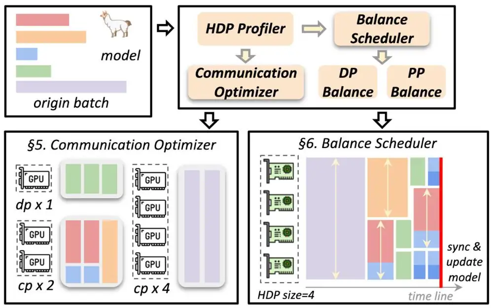
ByteScale has three parts (Figure 7 of the paper). A profiler builds cost models from the hardware, the model and the data. A communication optimizer decides how many ranks each sequence gets (sections 3.1–3.3), and a balance scheduler decides which rank runs which micro-batch (section 3.4).
ByteScale 有三個部分(論文 Figure 7)。profiler 依硬體、模型與資料建立成本模型。通訊最佳化器決定每條序列拿到多少 rank(第 3.1–3.3 節),平衡排程器決定哪個 rank 跑哪個 micro-batch(第 3.4 節)。
3.1 One pool of ranks: hybrid data parallelism3.1 一個 rank 池:混合資料平行
Hybrid data parallelism (HDP) replaces the DP × CP mesh with one pool of ranks, each holding up to tokens. A sequence longer than spans ranks, which pass K/V slices around their own ring. Shorter sequences are packed onto one rank by best fit and send nothing (Figure 2).
混合資料平行(HDP)用一個 個 rank 的池取代 DP × CP 網格,每個 rank 最多持有 個 token。比 長的序列跨 個 rank,沿自己的環傳遞 K/V 切片。較短的序列以 best fit 打包到一個 rank 上,什麼都不必送(圖 2)。
The pool also allows finer steps. At K a 768K sequence needs 96 ranks. On 128 ranks a static mesh must use ; HDP gives the sequence 96 ranks and the other 32 ranks an 8K sequence each.
這個池也讓分配更細。K 時,768K 的序列需要 96 個 rank。在 128 個 rank 上,靜態網格只能用 ;HDP 則給這條序列 96 個 rank,其餘 32 個 rank 各拿一條 8K 序列。
Creating NCCL communicators on the fly "incurs extra overhead", so ByteScale uses one global communicator over all HDP ranks for every P2P pair. HDP replicates weights and gradients as DP does and shards only the optimizer state (ZeRO-1). The gradient stays exact. DP sums the per-token gradients over the global batch (Eq. 1); HDP rank sums over the micro-batches of its share (Eq. 2):
臨時建立 NCCL communicator「會帶來額外開銷」,所以 ByteScale 對所有 P2P 配對都使用同一個涵蓋全部 HDP rank 的全域 communicator。HDP 像 DP 一樣複製權重與梯度,只把最佳化器狀態分片(ZeRO-1)。梯度也保持精確。DP 把全域批次 上每個 token 的梯度加總(Eq. 1);HDP 的 rank 加總它那一份 中各 micro-batch 的梯度(Eq. 2):
One all-reduce over all HDP ranks makes the two sums equal if the loss is scaled by the total token count (a token-level loss), not per sample. Then neither the spread of sequences nor the micro-batch count per rank changes the gradient; section 3.4 depends on this.
只要損失依總 token 數縮放(token 層級的損失),而不是依樣本縮放,在所有 HDP rank 上做一次 all-reduce 就能讓兩個總和相等。這時序列如何分散、每個 rank 跑幾個 micro-batch,都不會改變梯度;第 3.4 節就靠這一點。
3.2 Re-shaping the ring: when transfers hide behind attention3.2 重塑環:傳輸何時能藏在 attention 後面
In ring attention each of ranks receives one K/V slice per step while it computes on the previous one, so a step lasts . The transfer moves one rank's slice and depends only on . The compute does not: in a pack, each sequence is cut into slices, and a query attends only to its own sequence. With the time of one full block, our model is:
在 ring attention 中, 個 rank 每一步接收一個 K/V 切片,同時對前一個切片計算,所以一步的時間是 。傳輸 搬的是一個 rank 的切片,只取決於 。計算則不然:一包序列中的每條 都被切成 片,而 query 只關注自己那條序列。以 表示一個完整 區塊的時間,我們的模型是:
One sequence that fills the ring gives ; a pack of short sequences gives almost no compute but the same transfer. Figure 18(a) of the paper measured both cases (Figure 3). On the static 256-rank ring a step moved K/V in 1.4–1.6 ms against 0.30–0.42 ms of compute. Under HDP a 312K sequence used 39 ranks, and 2.8 ms of compute hid a 1.9 ms transfer. Both rings hold 8K tokens per rank; only the work per step differs. The paper does not say why the 39-rank transfer was slower.
一條填滿整個環的序列給出 ;一包短序列幾乎沒有計算,傳輸卻一樣多。論文 Figure 18(a) 量測了這兩種情況(圖 3)。在靜態的 256 rank 環上,每步傳送 K/V 花 1.4–1.6 ms,計算只有 0.30–0.42 ms。在 HDP 下,一條 312K 的序列用 39 個 rank,2.8 ms 的計算藏住了 1.9 ms 的傳輸。兩個環每個 rank 都持有 8K token;不同的只是每步的工作量。論文沒有說明為何 39 rank 環的傳輸比較慢。
The model applied to both measurements, one question per row:
把模型套用到兩個實測案例,逐列計算如下:
| Question問題 | Calculation算式 | Result結果 |
|---|---|---|
| Tokens per rank, static ring (2M context, 256 ranks)每個 rank 的 token,靜態環(2M 上下文、256 個 rank) | K | |
| Tokens per rank, HDP ring (312K sequence, 39 ranks)每個 rank 的 token,HDP 環(312K 序列、39 個 rank) | K | |
| Static ring: 255 transfers of about 1.5 ms, plus one compute block靜態環:255 次約 1.5 ms 的傳輸,加一個計算區塊 | msmeasured: 405 ms實測:405 ms | |
| HDP ring: 39 blocks of 2.8 ms; every 1.9 ms transfer hidesHDP 環:39 個 2.8 ms 的區塊;每次 1.9 ms 的傳輸都被隱藏 | msmeasured: 110 ms實測:110 ms | |
| P2P share of a baseline micro-batch (MLP 10 ms)基準 micro-batch 中 P2P 的比例(MLP 10 ms) | as the paper states與論文所述相同 |
The model matches both measurements within 6%. On the static ring, a pack of equal-length sequences hides its transfers only if : at the measured times, only for sequences of about 1.1M tokens or more. An HDP ring is filled by one sequence, so it hides its transfers whenever . The panel applies this to the whole length mix.
模型與兩個實測值的差距都在 6% 以內。在靜態環上,一包等長序列只有在 時才藏得住傳輸:以實測時間來算,只有約 1.1M token 以上的序列才行。HDP 的環由一條序列填滿,所以只要 就藏得住傳輸。面板把這套模型套用到整個長度分布。
3.3 Selective offloading: fewer ranks for a long sequence3.3 選擇性卸載:讓長序列用更少的 rank
A long sequence still needs many ranks, and each rank adds a ring step. So ByteScale moves part of a long sequence's activations to the much larger host memory. Activations are first in, last out: early layers can leave in the forward pass and return just in time for the backward pass. The copy is bytes against attention time, so it hides behind a long sequence's compute but not a short one's. It uses the DMA engines, not SMs, so it also overlaps NCCL traffic. For each sequence ByteScale picks the offload ratio that minimizes its rank count (Eq. 3). Here is the layers per rank, and are profiled cost models, and the copy bandwidths are profiled too:
長序列仍需要很多 rank,而每個 rank 都會多一個環步驟。所以 ByteScale 把長序列的一部分激活值移到大得多的主機記憶體。激活值是先進後出:前幾層可以在正向時移出,在反向剛好需要時移回。複製量是 位元組,attention 時間卻是 ,所以它藏得進長序列的計算,藏不進短序列的。複製使用 DMA 引擎而不是 SM,所以也能與 NCCL 流量重疊。對每條序列,ByteScale 選出讓 rank 數 最小的卸載比例 (Eq. 3)。其中 是每個 rank 的層數, 與 是量測得到的成本模型,複製頻寬也是量測而得:
The second line requires the copy to hide behind compute. In our reading, two layers stay on the GPU and a fraction of the other moves out, so gives and gives : a shorter ring, fewer P2P bytes and more free ranks.
第二行要求複製必須藏在計算後面。依我們的解讀,有兩層留在 GPU 上,其餘 層中有比例 移出,所以 時 , 時 :環更短、P2P 位元組更少、空出的 rank 更多。
3.4 The balance scheduler3.4 平衡排程器
HDP balances tokens, not time. ByteScale keeps micro-batches equal in tokens but lets ranks run different numbers of them (Figure 4). Algorithm 2 sorts the sequences by length into buckets of about equal FLOPs, then gives work to every rank that trails the slowest one by more than a threshold . DP-Balance (no PP) takes from the first bucket, so all ranks work on one length level at a time. PP-Balance takes from all buckets in turn: each pipeline gets one length level, so its stages stay in step, and pipelines with heavier micro-batches get fewer of them, so their total times meet at the sync. The token-level loss keeps both modes exact.
HDP 平衡的是 token,不是時間。ByteScale 讓 micro-batch 的 token 數相同,但允許各 rank 跑不同數量的 micro-batch(圖 4)。Algorithm 2 依長度把序列排序並分成 FLOPs 大致相等的桶,接著凡是落後最慢 rank 超過門檻 的 rank,都再分給它工作。DP-Balance(沒有 PP)從第一個桶取序列,所以所有 rank 同一時間處理同一個長度等級。PP-Balance 依序從所有桶取序列:每條管線拿到一個長度等級,讓各階段步調一致;micro-batch 較重的管線拿到較少的 micro-batch,使各管線的總時間在同步時對齊。token 層級的損失讓兩種模式都保持精確。
4. Implementation4. 實作
ByteScale is about 16K lines of Python, C++ and CUDA inside MegaScale, ByteDance's training framework. Ring attention uses the one global NCCL communicator and cuts each packed subsequence into chunks given out in front/back pairs, which balances the causal mask. Offloading uses separate CUDA streams and cached pinned host memory. A dataloader on Ray has one scheduler process that plans every step. The paper hides the GPUs, NICs and topology "due to business and confidential concerns".
ByteScale 約有 16K 行 Python、C++ 與 CUDA,建在字節跳動的訓練框架 MegaScale 之中。ring attention 使用那一個全域 NCCL communicator,把每條被打包的子序列切成 塊、以前後成對的方式分配,讓因果遮罩下的工作平均。卸載使用各自的 CUDA stream 與快取的 pinned 主機記憶體。跑在 Ray 上的資料載入器由一個排程行程規劃每一步。論文「基於商業與保密考量」隱藏了 GPU、NIC 與拓樸。
5. What was measured5. 量到了什麼
All runs are controlled benchmarks on the production cluster: LLaMA-7B, 13B, 30B and 70B on 1K, 2K, 4K and 8K GPUs, Mistral-8×7B on 8K and Mistral-8×22B on 16K, with the GitHub and Byted data at 256K to 2M context. The global batch is 32M tokens; throughput is the mean of 200 iterations after 20 warm-up iterations. The baseline is MegaScale with a static mesh, the smallest that fits, and the packed ring attention. "Naive" adds HDP with offloading; "balance" adds the scheduler. No error bars are given.
所有執行都是在生產叢集上的受控基準測試:LLaMA-7B、13B、30B、70B 分別用 1K、2K、4K、8K 顆 GPU,Mistral-8×7B 用 8K、Mistral-8×22B 用 16K,資料為 GitHub 與 Byted,上下文 256K 到 2M。全域批次為 32M token;吞吐取 20 次暖機後 200 次迭代的平均。基準是使用靜態網格的 MegaScale,採用裝得下的最小 ,並搭配打包 ring attention。「naive」加上帶卸載的 HDP;「balance」再加上排程器。論文沒有給誤差範圍。
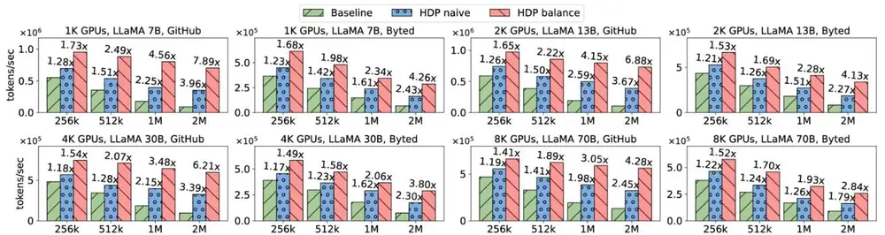
Speedups over the static mesh, read from the bar labels of Figure 17:
相對靜態網格的加速倍數,取自 Figure 17 的長條標籤:
| GPUs, model, contextGPU 數、模型、上下文 | Data資料 | Naive HDPNaive HDP | Balanced HDPBalanced HDP |
|---|---|---|---|
| 1,024 · LLaMA-7B · 2M | GitHub | 3.96× | 7.89× |
| 1,024 · LLaMA-7B · 2M | Byted | 2.43× | 4.26× |
| 8,192 · LLaMA-70B · 2M | GitHub | 2.45× | 4.28× |
| 16,384 · Mistral-8×22B · 2M | GitHub | 2.75× | 4.13× |
| 16,384 · Mistral-8×22B · 2M | Byted | 1.67× | 2.41× |
| all 12 panels · 256K全部 12 個子圖 · 256K | both兩者 | 1.12–1.28× | 1.28–1.73× |
The baseline's throughput fell about 2× per doubling of context; naive HDP fell 1.23× and balanced HDP 1.08× per doubling. At 2M on GitHub, the models without PP (DP-Balance) gained 6.21–7.89×, and those with PP (PP-Balance) 3.42–4.28×, because whole pipelines must balance. Byted gained less: 37% of its tokens (GitHub: 9.8%) sit in sequences over 256K, which need large rings in any layout.
基準的吞吐在上下文每加倍一次時約降 2 倍;naive HDP 每次降 1.23 倍,balanced HDP 降 1.08 倍。在 GitHub 2M 時,沒有 PP 的模型(DP-Balance)加速 6.21–7.89 倍,有 PP 的模型(PP-Balance)加速 3.42–4.28 倍,因為必須平衡整條管線。Byted 加速較少:它有 37% 的 token(GitHub 為 9.8%)位在超過 256K 的序列中,這些序列不論怎麼配置都需要大的環。
Figure 18 follows one step of LLaMA-7B (2M context, 1,024 GPUs, Byted data). Under naive HDP, four sampled ranks finished between 1m41s and 4m32s, so one idled 171 s; with balancing all four finished at 2m36s–2m37s. Over all 1,024 ranks (Figure 18c), naive per-rank computation took 60 to 279 s. Its longest was 1.7× shorter than the baseline's, and balancing cut it a further 2.3×.
Figure 18 追蹤 LLaMA-7B 的一步(2M 上下文、1,024 顆 GPU、Byted 資料)。naive HDP 下,抽樣的四個 rank 在 1 分 41 秒到 4 分 32 秒之間完成,所以有一個閒置了 171 秒;加上平衡後,四個都在 2 分 36 秒到 2 分 37 秒完成。在全部 1,024 個 rank 上(Figure 18c),naive 的每 rank 計算時間介於 60 到 279 秒。它最長的時間比基準短 1.7 倍,平衡又再縮短 2.3 倍。
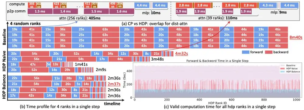
The step times of Figure 18(b) give these ratios:
由 Figure 18(b) 的步驟時間可得以下比值:
| Question問題 | Calculation算式 | Result結果 |
|---|---|---|
| Baseline step over naive step (8m40s, 4m32s)基準一步對 naive 一步(8 分 40 秒、4 分 32 秒) | ||
| Baseline step over balanced step (2m37s)基準一步對 balanced 一步(2 分 37 秒) |
Two figures disagree. The ablation (Figure 20) claims the same configuration and gives cumulative gains of 1.59× (dynamic communication), 2.01× (+ offloading), 3.69× (+ balance) and 3.89× (+ remote dataloader). Figure 17 gives 2.43× and 4.26× for it. The final throughputs agree (about 2.9 × 10⁵ tokens/s); the baselines do not (about 0.67 vs 0.74 × 10⁵). Read each speedup as one run, uncertain by about 10%.
兩張圖互相矛盾。消融實驗(Figure 20)宣稱用相同的配置,給出累計的 1.59 倍(動態通訊)、2.01 倍(+ 卸載)、3.69 倍(+ 平衡)與 3.89 倍(+ 遠端資料載入器)。Figure 17 對同一配置給出 2.43 倍與 4.26 倍。兩者的最終吞吐一致(約每秒 2.9 × 10⁵ token),基準卻不一致(約 0.67 對 0.74 × 10⁵)。請把每個加速倍數都當成誤差約 10% 的單次執行。
A two-hour trace (Figure 19) shows the network side. Peak RDMA output fell from about 110 to about 65 Gb/s with naive HDP and became steady with balancing, while tensor-core activity rose from about 10% to about 40%; the paper does not say whether traffic is per NIC or per node. At 64K context (Figure 21), cut memory from 59 to 40 GB at no cost; reached 27 GB but cost about 28%, close to recomputation's 32%.
一段兩小時的紀錄(Figure 19)顯示網路這一側。naive HDP 讓 RDMA 輸出峰值從約 110 降到約 65 Gb/s,加上平衡後變得平穩,而 tensor core 的使用率從約 10% 升到約 40%;論文沒有說明流量是每張 NIC 還是每個節點。在 64K 上下文(Figure 21)下, 把記憶體從 59 GB 降到 40 GB 而沒有代價; 降到 27 GB,但代價約 28%,接近重算的 32%。
6. Limits and open questions6. 限制與未解的問題
The paper has no limitations section. A careful reader should ask:
論文沒有限制一節。細心的讀者應該追問:
- Hardware. GPUs, NIC speed and topology are hidden, so the ring-step times cannot be turned into bandwidth or placed on a network tier.硬體。GPU、NIC 速度與拓樸都被隱藏,所以環步驟時間既無法換算成頻寬,也無法對應到網路的哪一層。
- Baseline. The static mesh is the design HDP improves on; there is no comparison with Ulysses-style sequence parallelism, all-gather CP, or the variable-length systems the paper cites.基準。靜態網格正是 HDP 要改進的設計;論文沒有與 Ulysses 式序列平行、all-gather CP 或它引用的變長序列系統比較。
- Spread. 7.89× is the best of 48 cells (production data at 16,384 GPUs: 2.41×), each point is one run, and Figures 17 and 20 differ by about 10%.差距。7.89 倍是 48 格中最好的一格(16,384 顆 GPU 的生產資料為 2.41 倍),每個點都是單次執行,Figure 17 與 Figure 20 相差約 10%。
- Network and host. Rings change every step, and so does the traffic matrix; how ECMP or adaptive routing copes is not studied. PCIe contention between offload copies and the NIC is not measured.網路與主機。環每一步都在變,流量矩陣也跟著變;ECMP 或自適應路由如何應對沒有研究。卸載複製與 NIC 在 PCIe 上的爭用也沒有量測。
- Control path and convergence. The cost of one scheduler process planning every step for 16,384 GPUs is not measured, and no loss curves are shown.控制路徑與收斂。一個排程行程為 16,384 顆 GPU 規劃每一步的成本沒有量測,也沒有給出損失曲線。
7. How it connects7. 與其他內容的關聯
- Deep dive, sections 5–6: CP need not be one degree per job. The order [TP, CP, PP, DP] still holds, but CP and DP become one dimension whose groups change every step.第 3 章第 5–6 節:CP 不必每個任務只有一個度數。[TP, CP, PP, DP] 的順序仍成立,但 CP 與 DP 合成一個維度,它的群組每一步都在變。
- Deep dive, section 4 and Panel 4: the bubble formula assumes equal micro-batches; ByteScale removes the bubble of unequal ones with unequal counts.第 3.5 節與面板 4:氣泡公式假設 micro-batch 都相等;ByteScale 以不相等的數量消除不相等 micro-batch 造成的氣泡。
- Llama 3 used a static CP of 16 with front/back chunks; ByteScale pairs chunks the same way per subsequence but sizes the ring per sequence. MegaScale is its host framework and baseline.Llama 3 用靜態的 CP 16 與前後成對的切塊;ByteScale 對每條子序列同樣成對切塊,但逐序列決定環的大小。MegaScale 是它所在的框架與基準。
- Rail-only and Alibaba HPN: if TP stays inside a server, ring partners share a local rank, so ring traffic stays on a rail (our inference; the paper is silent on topology).Rail-only 與 Alibaba HPN:如果 TP 留在伺服器內,環上的夥伴具有相同的本地 rank,環上流量就留在同一條 rail(我們的推論;論文對拓樸沒有著墨)。
- The PipeMorph digest: uneven micro-batch timing from a slow link there, from data here; both change per-pipeline counts and use host memory as slack. Balancing and Beyond and UBEP show data-made skew for experts.PipeMorph 導讀:那裡的 micro-batch 時間因慢鏈路而不均,這裡因資料而不均;兩篇都改變每條管線的數量,並拿主機記憶體當餘裕。Balancing and Beyond 與 UBEP 則呈現專家上由資料造成的偏斜。
Key numbers關鍵數字
| Number | 數字 | Meaning (production cluster, hardware undisclosed) | 意義(生產叢集,硬體未公開) |
|---|---|---|---|
| 1% / 44.3% | Byted samples at 128K or longer / their token share (dataset statistic) | Byted 中 128K 以上的樣本 / 它們的 token 占比(資料集統計) | |
| 405 → 110 ms | One attention module: 256-rank static ring → 39-rank HDP ring | 一個 attention 模組:256 rank 靜態環 → 39 rank HDP 環 | |
| 1.4–1.6 vs 0.30–0.42 ms | P2P vs compute per step, static ring (HDP ring: 1.9 vs 2.8 ms) | 每步的 P2P 對計算,靜態環(HDP 環:1.9 對 2.8 ms) | |
| 8m40s → 4m32s → 2m37s | One step: baseline → naive → balanced; LLaMA-7B, 2M, 1,024 GPUs | 一步:基準 → naive → balanced;LLaMA-7B、2M、1,024 顆 GPU | |
| 7.89× / 4.26× | Best speedup, GitHub / Byted; same setup | 最佳加速,GitHub / Byted;設定同上 | |
| 4.13× / 2.41× | GitHub / Byted, Mistral-8×22B on 16,384 GPUs, 2M | GitHub / Byted,Mistral-8×22B 在 16,384 顆 GPU 上,2M | |
| 3.89× vs 4.26× | Full system, Figure 20 vs Figure 17, one stated configuration | 完整系統,Figure 20 對 Figure 17,宣稱為同一配置 |
Terms used on this page本頁用到的術語
- Hybrid data parallelism (HDP)
- One pool of ranks with up to tokens each; a sequence spans of them.
- 一個 個 rank 的池,每個最多 個 token;一條序列跨其中 個。
- Token-level loss
- A loss scaled by the total token count, so the gradient ignores how tokens are spread over ranks.
- 依總 token 數縮放的損失,使梯度與 token 如何分散到各 rank 無關。
- Selective offloading
- Moving a fraction of a long sequence's activations to host memory, so it needs ranks instead of .
- 把長序列比例 的激活值移到主機記憶體,讓它只需要 而非 個 rank。
- DP-Balance / PP-Balance
- Scheduler modes that balance work per time step (no PP) or total time per pipeline (with PP).
- 平衡每個時間步的工作(沒有 PP)或每條管線總時間(有 PP)的排程模式。