Matrix Sweep: Agentic KV Scheduling Across GPUs

1. Experiment Setup

1.1 Hardware

1.2 Model & dataset

Tool distribution

Each SWE-smith trajectory is an OpenAI-format chat log: a system prompt, the issue description as the user message, and alternating assistant / tool turns. A worked example showing the JSON structure together with its per-turn token budget lives in §2.1.

1.3 Scheduling policies tested

1.4 Arrival rate sweep

Jobs arrive as a Poisson process. JPS (jobs per second) values: 1, 3, 6, 10. Each job runs its full ~18-turn trajectory; between turns a 1-second synthesized tool-exec delay is inserted to emulate real agent loop back-pressure.

2. Per-turn prefill / decode token budget

Every chat turn of a job goes through exactly two phases inside the vLLM engine:

• Prefill — one forward pass over the input tokens that are not already in the prefix cache. Counts as ≥ 1 step (1 if all uncached tokens fit in max_num_batched_tokens, otherwise split into chunked-prefill steps).
• Decode — each forward pass emits exactly one token. N output tokens ⇒ N decode steps.

Minimum engine steps for a single turn = 1 (prefill, ≥ 1 if chunked) + N (one per decoded token) = 1 + num_output_tokens.

2.1 Worked example — astropy__astropy-12907 turn 2

The trajectory (abridged) and the token accounting for turn 2 share one block below. Counts are representative (Llama-3.1 tokenizer).

# ── Trajectory (abridged, 2 of ~17 turns shown) ──────────────────────────
{
  "instance_id": "astropy__astropy-12907",
  "messages": [
    {"role": "system",
     "content": "You are a SWE agent. Use the tools to explore the repo and fix the issue…"},

    {"role": "user",
     "content": "<issue>Modeling's `separability_matrix` does not compute separability correctly for nested CompoundModels</issue><repo>astropy/astropy</repo>"},

    // turn 1 — explore
    {"role": "assistant",
     "content": "Let me look at the modeling package.",
     "tool_calls": [{"id": "c1", "type": "function",
       "function": {"name": "cd", "arguments": "{\"path\": \"astropy/modeling\"}"}}]},
    {"role": "tool", "tool_call_id": "c1", "content": "/astropy/modeling"},

    // turn 2 — read the suspect file   ← the turn we score below
    {"role": "assistant",
     "content": "Opening separable.py to inspect _separable().",
     "tool_calls": [{"id": "c2", "type": "function",
       "function": {"name": "editor_view", "arguments": "{\"path\": \"separable.py\", \"view_range\": [1, 120]}"}}]},
    {"role": "tool", "tool_call_id": "c2",
     "content": "def _separable(transform): …  # ~115 lines of source"},

    // … 15 more turns (editor_str_replace, editor_view, editor_str_replace, submit) …
  ]
}

# ── Turn 2 · Input side — prompt_tokens fed to the engine ────────────────
  system prompt                              …   604 tok
  user (issue body + reproduction code)      … 1,498 tok
  turn 1 assistant text + tool_calls JSON    …    35 tok
  turn 1 synthesized ```bash cd ```          …     5 tok
  turn 1 tool response "/astropy/modeling"   …    10 tok
  turn 2 assistant role prefix               …     3 tok
                                             ─────────
  prompt_tokens (prefill input)           = 2,155 tok

# ── Turn 2 · Output side — tokens generated during decode ────────────────
  "Opening separable.py to inspect _separable()."        → 10 tok
  tool_calls JSON (editor_view, separable.py, 1..120)    → 13 tok
  synthesized ```bash\neditor_view\n```                  →  5 tok
                                                         ─────────
  output_tokens                                       =    28 tok

# ── Turn 2 · Minimum engine steps ────────────────────────────────────────
  prefill   : 1 step   (2,155 ≤ max_num_batched_tokens = 8,192 → one forward pass)
  decode    : 28 steps (one forward pass per emitted token)
                                               ─────────
  min steps                             = 29 steps
  general form: 1 + num_output_tokens

2.2 Synthesized tool-call injection

Continuum's pin estimator classifies the upcoming tool by parsing a trailing ```bash\n<tool_name>\n``` block in the assistant's content. Raw SWE-smith trajectories carry tools in the OpenAI tool_calls field instead, so a preprocessor synthesizes that bash block from tool_calls[0].function.name before tokenization — the extra 5 tokens shown in the example above.

3. Results — Summary Table (avg job duration, seconds)

Below: mean total turn duration per job including queue wait, across 100 jobs × ~18 turns. Lower = better. Bold highlights per-row winner.

H100 80GB

A100 PCIE 40GB / 80GB (mixed — see annotations)

H200 141GB

3.1 H100 80GB — 9-chart panel

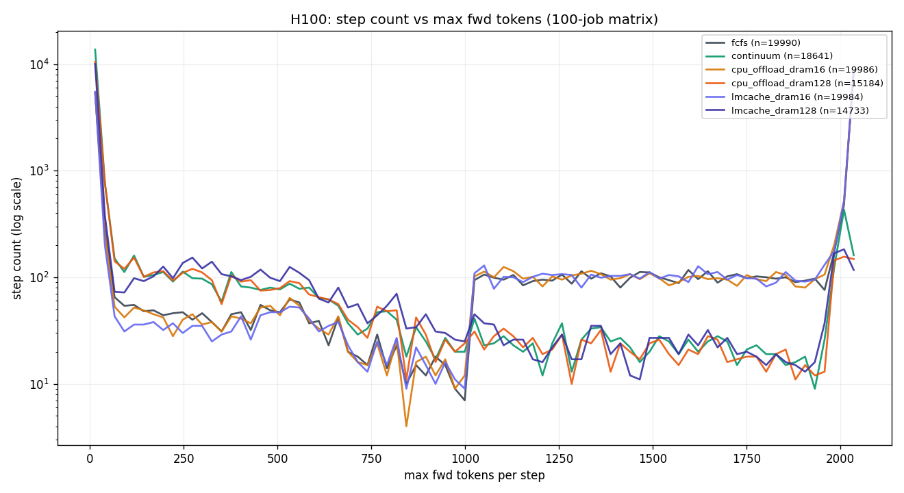
Fig. H100-a — Histogram of max forward tokens per scheduler step across all policies (log-scale y). The dominant cluster at 1–4 tokens = decode steps. The budget-cap spike at 2048 = prefill-heavy steps hitting max_num_scheduled_tokens. Continuum and cpu_offload_128G show tighter distributions; cpu_offload_16G and lmcache_16G have heavier right tails due to prefill retries after eviction.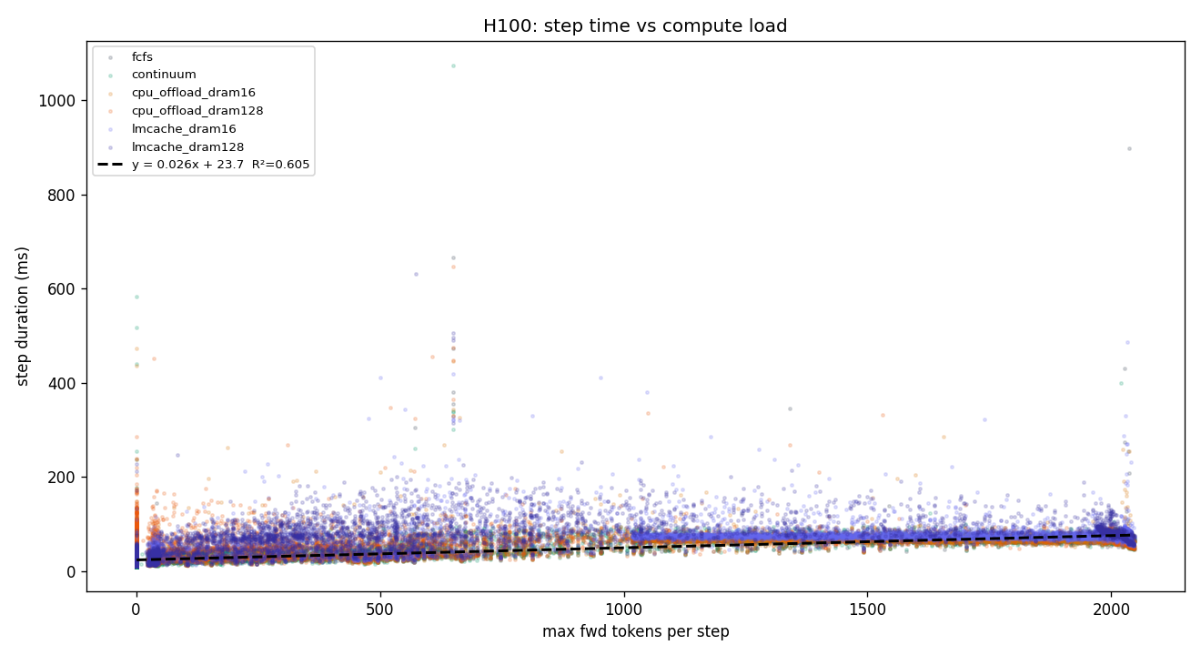

Fig. H100-b — Per-step scatter: x = max fwd tokens, y = measured step duration (ms). Global linear regression: y = 0.0258·x + 23.7, R² = 0.605. Interpretation: each additional token costs ~26 μs of step time; the 24 ms intercept is fixed per-step overhead (kernel launch + scheduler + Python dispatch).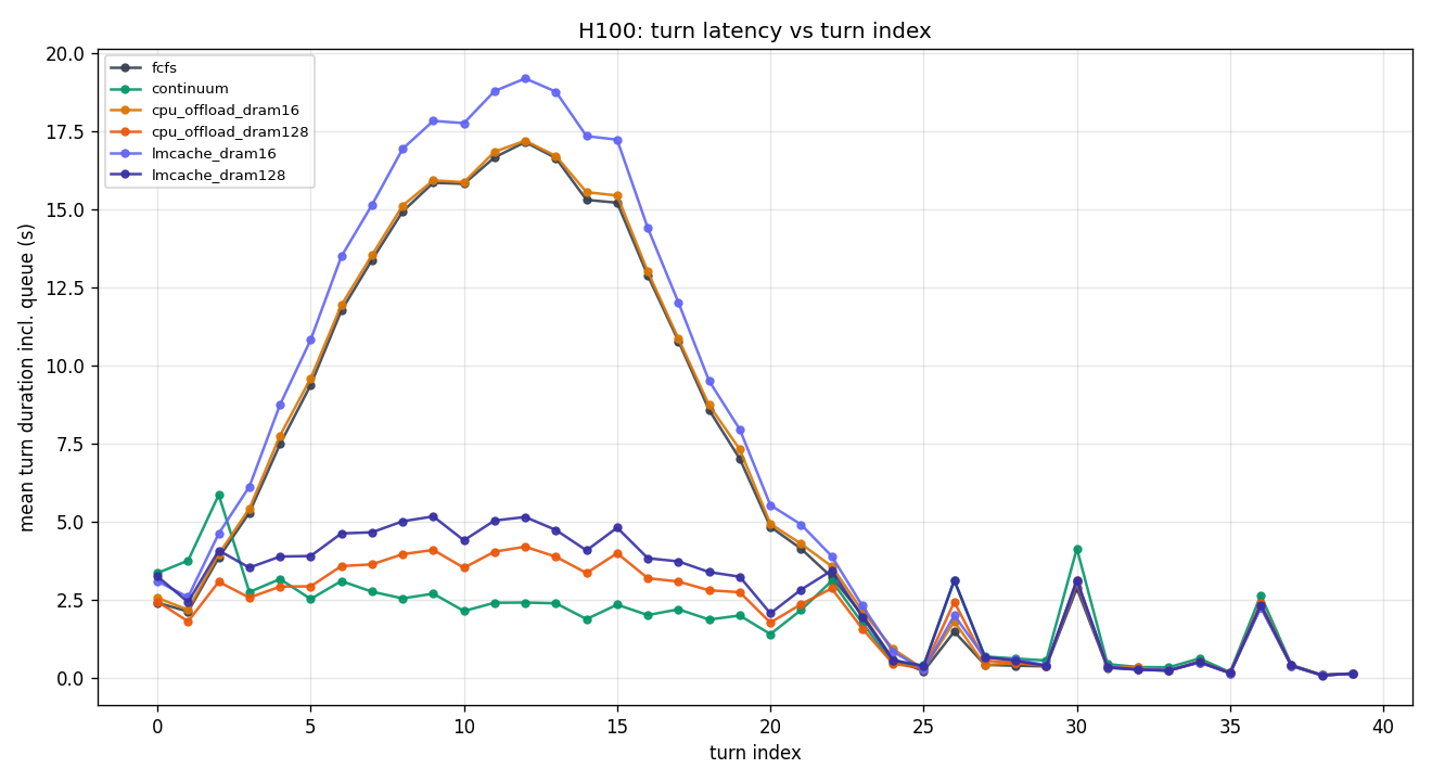

Fig. H100-c — Per-turn mean duration (including queue wait), colored by policy. FCFS / cpu_offload_16G / lmcache_16G show the classic queue-buildup pattern: later turns hit progressively longer queues as concurrent jobs accumulate. Continuum and cpu_offload_128G stay flat, indicating KV reuse successfully prevents rework.

3.2 A100 PCIE 40GB — 9-chart panel

Fig. A100-a — A100 histogram. With only ~90K KV tokens, chunked-prefill fragmentation is extreme: lmcache_16G shows a broad secondary peak around 256 tokens (constant small-chunk prefill). Continuum shifts left-heavy (decode-dominated) because pinning retains prefix blocks across turns.

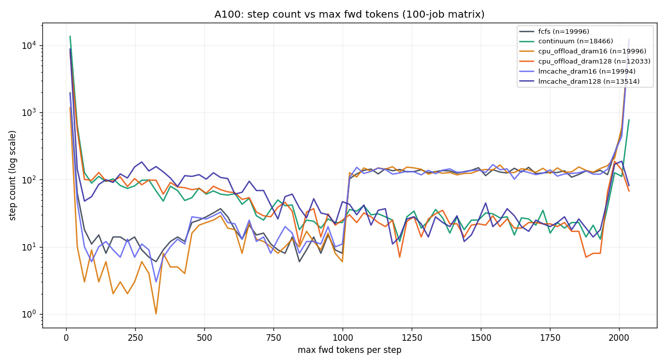
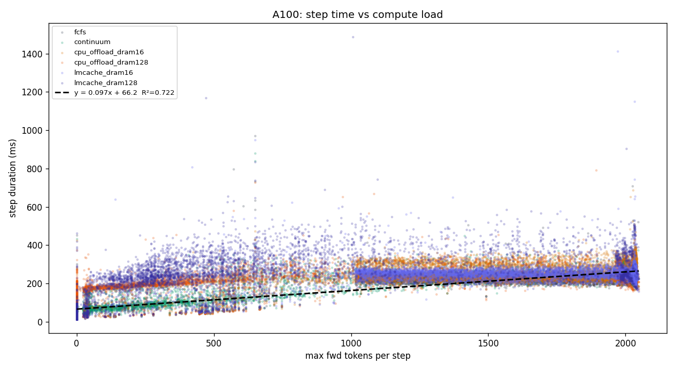
Fig. A100-b — A100 regression: y = 0.0973·x + 66.2 ms, R² = 0.722. A100 is 3.8× slower per token than H100 (26 μs → 97 μs) and has 2.8× higher per-step overhead (24 → 66 ms) — reflecting slower PCIe 4.0 + weaker TensorCore throughput.

Fig. A100-c — A100 reveals the full policy spectrum. FCFS collapses (>700 s by turn 15). lmcache_16G / cpu_offload_16G are even worse due to slow PCIe 4.0 KV transfers on cache misses. Continuum and cpu_offload_128G hold the line at ~250 s asymptote. On tight-KV GPUs, smart policy is the difference between 4× and 15× slowdown at JPS ≥ 3.

3.3 H200 141GB — 9-chart panel

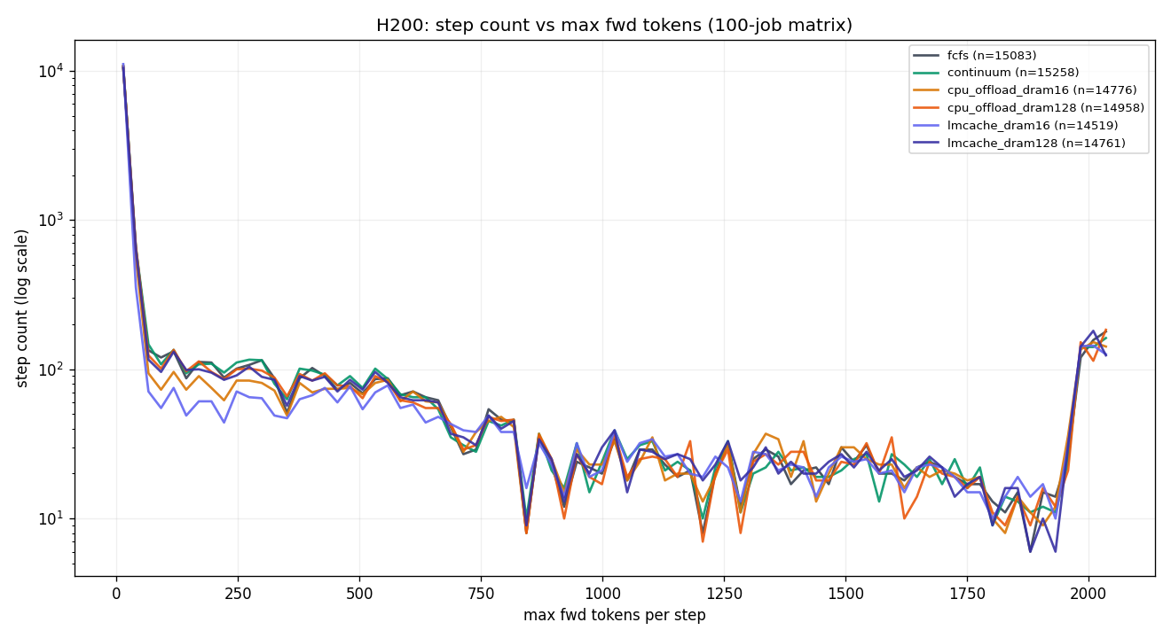
Fig. H200-a — H200 histogram. All policies converge into a near-identical shape because the 141 GB KV cache fits essentially the entire working set. lmcache_16G is the only outlier — deliberately tight DRAM forces external-cache thrash even when GPU KV is plentiful.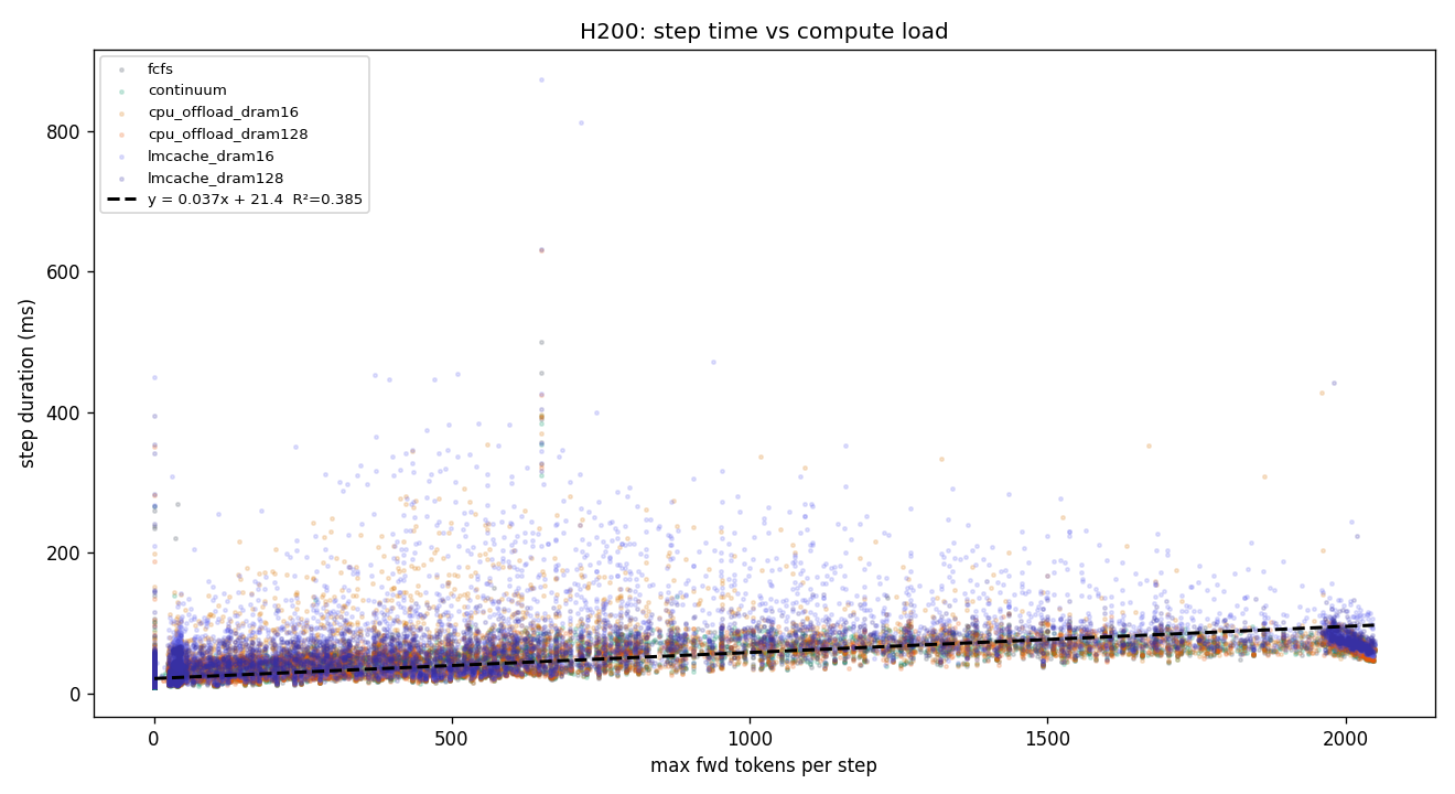

Fig. H200-b — H200 regression: y = 0.0371·x + 21.4 ms, R² = 0.385. Notably lower R² than H100/A100 — compute is so fast that per-step variance is dominated by non-compute factors (scheduler overhead, I/O, Python GIL), not max fwd tokens. Per-token cost (37 μs) is 1.4× H100's, but intercept (21 ms) is actually lower — H200's kernel launch overhead is smaller.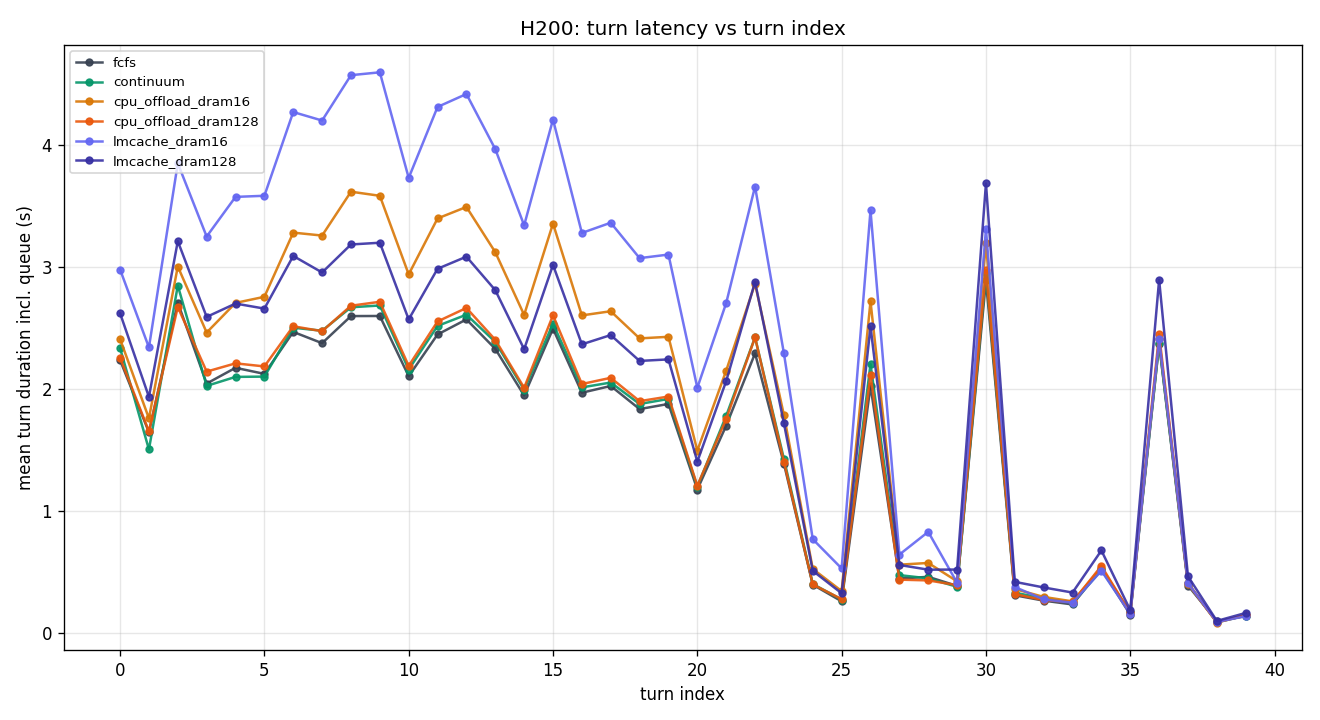

Fig. H200-c — H200 turn-latency: almost flat for all policies except lmcache_16G and cpu_offload_16G (which still suffer from forced eviction). Confirms that policy matters only when KV pressure exists.

4. Regression Analysis — Compute Cost Model

Fitting step_duration = slope·max_fwd_tokens + intercept across all policies on each GPU:

5. Takeaways

5.1 Engineering issues surfaced by this matrix

• Scheduler assertion crash under heavy KV pressure (A100 40GB + Continuum): vllm/v1/core/sched/scheduler.py:1021 asserts sum(scheduled_*_req_ids) ≤ len(self.running). Under extreme contention the invariant temporarily breaks. Downgraded to a warning; no downstream effect observed.
• vLLM cache grows in $HOME silently: vLLM writes ~10 GB of compile cache into ~/.cache/vllm, which overflows PACE's 20 GB home quota after ~5 runs. Root cause: XDG_CACHE_HOME alone is insufficient — vllm hardcodes Path.home() / '.cache' / 'vllm'. Fix: export VLLM_CACHE_ROOT=<scratch-dir>/vllm alongside XDG_CACHE_HOME.
• SimpleCPUOffloadConnector extra_config key: Docs reference cpu_kv_cache_size_bytes; actual code reads cpu_bytes_to_use_per_rank. Using the wrong key silently caps CPU KV at 0, forcing GPU-only behavior.
• Slurm default --gres=gpu:1 can route to V100: V100 (sm_70) cannot load vLLM 0.19 (FlashAttention 2 requires sm_80+). Must pin --gres=gpu:h100:1 or :a100:1 explicitly.

5.2 What we did not measure (limitations)

• Tool exec delay is uniform 1 s. Real tools (find/grep/python) span 0.01 s (cd) to 60 s (pytest). A per-tool-type distribution would test Continuum's dynamic pin-TTL more faithfully.
• No long-context (>16K) jobs included. Llama-3.1-8B supports 128K; tight-KV GPUs would be hit even harder and policy gaps would widen.
• Each run used a single GPU. Tensor parallel / pipeline parallel interactions with Continuum pin are untested.
• No correctness validation. Forced decoding by construction reproduces recorded tokens; a real-agent replay (sampling-free) would surface scheduling-induced quality drift if any.

7. Interactive Trace Viewer

Every run produces per-step JSONL traces (step_snapshot + step_decision + prefix_cache_lookup). Load them into the interactive scheduler trace viewer to inspect individual steps, prefill/decode phases, KV block allocation, pin state, and admission limits.

Viewer features

• Per-step running/waiting queue with pill badges: category (new/running/resumed/preempted/skipped), turn index, KV blocks held, decode age
• Prefill progress: [prefill:Nb(Mt), Tt total, P% cached, fwd:Xt]
• VRAM block info: free / used (split into pin + active) / total
• DRAM block info (CPU offload / LMCache runs)
• Token budget: tok:X/Y with admission-limit reason badges (tok-budget, kv-insuf, max-seqs)
• Prefix cache hit per request: hit:N/M(P%) with local/external split when connector is present
• Pin list with job IDs, de-duplicated per job