Learning Objectives
By the end of this lab, you will be able to:
- Explain the fundamental tension in co-located serving: prefill is compute-bound and decode is memory-bandwidth-bound, leading to mutual interference under mixed traffic
- Configure vLLM disaggregated prefill/decode using two H100 instances connected with P2pNcclConnector
- Measure TTFT vs input length for both standard and disaggregated serving modes to quantify TTFT improvement
- Compare disaggregated P/D against TP=2 standard serving to understand when disaggregation is preferable
- Examine the KV transfer path in vllm/distributed/kv_transfer/ and sglang/srt/disaggregation/ to understand protocol design
Key Concepts
KV Transfer Flow in vLLM P2pNcclConnector
- After P instance finishes prefill, it has a full KV cache for the request (shape: [num_layers, 2, num_heads, seq_len, head_dim])
- P2pNcclConnector sends KV pages to D instance via ncclSend/ncclRecv using the pre-established NCCL communicator between GPU 0 and GPU 1
- D instance receives KV tensors into its own KV cache pool and immediately starts decode — no recomputation needed
- The KV transfer adds latency proportional to sequence length; for Llama-8B at TP=1, transferring 1K tokens of KV takes ~2-5 ms over NVLink
Disagg P/D vs TP=2: Different Tradeoffs
- TP=2 standard — both GPUs collaborate on every single request (prefill and decode). Reduces per-token latency via parallelism but still suffers from prefill-decode contention at co-location.
- Disagg P/D — each GPU is specialized. P GPU runs only prefill at maximum compute utilization; D GPU runs only decode with maximum KV cache capacity. Completely eliminates prefill-decode interference at the cost of KV transfer overhead and 2× total GPU usage per request.
Setup & Configuration
# Verify 2× H100 GPUs are visible
nvidia-smi --query-gpu=index,name,memory.total --format=csv,noheader

# Check NVLink connectivity between GPU 0 and GPU 1
nvidia-smi topo -m

# Verify vLLM version supports disaggregated P/D (requires >= 0.6.0)
python -c "import vllm; print(vllm.__version__)"

# Verify the kv_transfer module is present
python -c "from vllm.distributed.kv_transfer.kv_connector.factory import KVConnectorFactory; print('OK')"

# Download model weights if not cached
python -c "from huggingface_hub import snapshot_download; snapshot_download('meta-llama/Llama-3.1-8B-Instruct')"
Experiments
Standard Co-located Serving Baseline (1 GPU)
Establish baseline TTFT under mixed long-prefill and short-decode traffic on a single GPU. This demonstrates the prefill-decode interference problem:
# Standard vLLM on GPU 0 only (TP=1, co-located P+D)
CUDA_VISIBLE_DEVICES=0 vllm serve meta-llama/Llama-3.1-8B-Instruct \
  --port 8000 \
  --tensor-parallel-size 1 \
  --disable-log-requests &
sleep 30

# Measure TTFT across input lengths 128, 512, 1024, 2048 tokens
python - <<'PYEOF'
import time, requests

URL = "http://localhost:8000/v1/chat/completions"
MODEL = "meta-llama/Llama-3.1-8B-Instruct"

def make_prompt(n_words):
    return "Context: " + ("The quick brown fox jumps over the lazy dog. " * (n_words // 9))

INPUT_CONFIGS = {
    128:  make_prompt(90),
    512:  make_prompt(365),
    1024: make_prompt(730),
    2048: make_prompt(1460),
}

print(f"{'input_len':>10} | {'ttft_ms p50':>12} | {'ttft_ms p99':>12}")
print("-" * 42)
for approx_tokens, prompt in INPUT_CONFIGS.items():
    ttfts = []
    for _ in range(10):
        t0 = time.perf_counter()
        requests.post(URL, json={
            "model": MODEL,
            "messages": [{"role": "user", "content": prompt + " Summarize briefly."}],
            "max_tokens": 30}, timeout=300)
        ttfts.append((time.perf_counter() - t0) * 1000)
    s = sorted(ttfts)
    print(f"{approx_tokens:>10} | {s[4]:>12.1f} | {s[-1]:>12.1f}")
PYEOF

kill %1; sleep 10Disaggregated P/D with vLLM P2pNcclConnector
The commands below are documented for reference but will fail on PACE's single-node 2-GPU topology with RuntimeError: Engine core initialization failed. Failed core proc(s): {}. The P2pNcclConnector is designed for multi-node production deployments (one GPU per instance per node, LB + connector over TCP), not for two GPUs sharing a single NCCL channel on the same host. See the Results section below for the disclosed failure and the TP=1 / TP=2 bracketing we used as upper/lower bounds instead.
Launch two vLLM instances — one Prefill-only on GPU 0 and one Decode-only on GPU 1 — with P2pNcclConnector for KV transfer. The disaggregated LB proxy routes requests automatically:
# Terminal 1: Prefill instance on GPU 0
CUDA_VISIBLE_DEVICES=0 vllm serve meta-llama/Llama-3.1-8B-Instruct \
  --port 8100 \
  --tensor-parallel-size 1 \
  --kv-transfer-config '{
    "kv_connector": "PyNcclConnector",
    "kv_role": "kv_producer",
    "kv_rank": 0,
    "kv_parallel_size": 2,
    "kv_buffer_device": "cuda",
    "kv_buffer_size": 1e9
  }' \
  --disable-log-requests &

# Terminal 2: Decode instance on GPU 1
CUDA_VISIBLE_DEVICES=1 vllm serve meta-llama/Llama-3.1-8B-Instruct \
  --port 8200 \
  --tensor-parallel-size 1 \
  --kv-transfer-config '{
    "kv_connector": "PyNcclConnector",
    "kv_role": "kv_consumer",
    "kv_rank": 1,
    "kv_parallel_size": 2,
    "kv_buffer_device": "cuda",
    "kv_buffer_size": 1e9
  }' \
  --disable-log-requests &
sleep 40

# Measure TTFT across same input lengths — compare with baseline
python - <<'PYEOF'
import time, requests

PREFILL_URL = "http://localhost:8100/v1/chat/completions"
DECODE_URL  = "http://localhost:8200/v1/chat/completions"
MODEL = "meta-llama/Llama-3.1-8B-Instruct"

def make_prompt(n_words):
    return "Context: " + ("The quick brown fox jumps over the lazy dog. " * (n_words // 9))

INPUT_CONFIGS = {
    128:  make_prompt(90),
    512:  make_prompt(365),
    1024: make_prompt(730),
    2048: make_prompt(1460),
}

print(f"{'input_len':>10} | {'ttft_ms p50':>12} | {'ttft_ms p99':>12}")
print("-" * 42)
for approx_tokens, prompt in INPUT_CONFIGS.items():
    ttfts = []
    for _ in range(10):
        t0 = time.perf_counter()
        requests.post(PREFILL_URL, json={
            "model": MODEL,
            "messages": [{"role": "user", "content": prompt + " Summarize briefly."}],
            "max_tokens": 30}, timeout=300)
        ttfts.append((time.perf_counter() - t0) * 1000)
    s = sorted(ttfts)
    print(f"{approx_tokens:>10} | {s[4]:>12.1f} | {s[-1]:>12.1f}")
PYEOF

kill %1 %2; sleep 10TTFT vs Input Length: Standard vs Disaggregated
Plot TTFT as a function of input prompt length for both configurations. The key observation: in disaggregated mode, TTFT grows more slowly with input length because the P instance is uncontested by decode traffic:
# Collect data points for the TTFT-vs-input-length plot
# Run Exp 1 (standard) and Exp 2 (disagg) with extended sweep

INPUT_LENGTHS = [64, 128, 256, 512, 768, 1024, 1536, 2048]

# For each config, report the column-by-column comparison:
# input_len | standard_p50_ms | disagg_p50_ms | improvement_%

python - <<'PYEOF'
# (Run this after both server pairs are up from Exp 1 and Exp 2 data)
import json

results_standard = {}   # fill from Exp 1 logs
results_disagg   = {}   # fill from Exp 2 logs

print(f"{'input_len':>10} | {'std_p50':>9} | {'disagg_p50':>10} | {'improvement':>11}")
print("-" * 50)
for n in [128, 512, 1024, 2048]:
    std  = results_standard.get(n, float('nan'))
    dis  = results_disagg.get(n,   float('nan'))
    impv = (std - dis) / std * 100 if std and dis else float('nan')
    print(f"{n:>10} | {std:>9.1f} | {dis:>10.1f} | {impv:>10.1f}%")
PYEOFTP=2 Standard Serving Comparison
Compare disaggregated P/D (1 GPU each) against TP=2 standard serving (both GPUs collaborate on every request). This clarifies when you should prefer disaggregation vs tensor parallelism for a 2-GPU budget:
# TP=2 standard baseline (both GPUs, co-located P+D)
vllm serve meta-llama/Llama-3.1-8B-Instruct \
  --port 8000 \
  --tensor-parallel-size 2 \
  --disable-log-requests &
sleep 40

python - <<'PYEOF'
import time, requests

URL   = "http://localhost:8000/v1/chat/completions"
MODEL = "meta-llama/Llama-3.1-8B-Instruct"

configs = {
    "short_input_short_output":  ("Hello, how are you? " * 5,  20),
    "long_input_short_output":   ("Context: " + "Lorem ipsum dolor sit amet. " * 70, 30),
    "short_input_long_output":   ("Write a detailed essay on neural networks.",    200),
}

print(f"{'workload':40} | {'ttft_ms':>8} | {'e2e_ms':>8}")
print("-" * 65)
for label, (prompt, max_tok) in configs.items():
    ttfts, e2es = [], []
    for _ in range(8):
        t0 = time.perf_counter()
        r  = requests.post(URL, json={"model": MODEL,
            "messages": [{"role": "user", "content": prompt}],
            "max_tokens": max_tok}, timeout=300)
        e2e = (time.perf_counter() - t0) * 1000
        e2es.append(e2e)
    print(f"{label:40} | {sorted(e2es)[3]:>8.1f} | {sorted(e2es)[-1]:>8.1f}")
PYEOF

kill %1; sleep 10KV Transfer Profiling — Overhead Measurement
Estimate the NCCL P2P KV transfer time between GPU 0 and GPU 1 as a function of sequence length. This overhead is the primary cost of disaggregation vs co-location:
# Estimate KV size: for Llama-8B (32 layers, 32 KV heads, head_dim=128, BF16)
# KV per token = 2 (K+V) * 32 layers * 32 heads * 128 * 2 bytes = 524,288 bytes = 512 KB
python - <<'PYEOF'
import torch

LAYERS   = 32
KV_HEADS = 32
HEAD_DIM = 128
BYTES    = 2  # BF16

for seq_len in [64, 128, 256, 512, 1024, 2048]:
    kv_bytes = 2 * LAYERS * KV_HEADS * seq_len * HEAD_DIM * BYTES
    kv_mb    = kv_bytes / 1e6
    # NVLink: ~900 GB/s aggregate, P2P = ~600 GB/s effective
    nvlink_ms = kv_bytes / (600e9 / 1000)
    print(f"seq_len={seq_len:5d}  KV_size={kv_mb:6.1f} MB  "
          f"est_NVLink_transfer={nvlink_ms:.2f} ms")
PYEOF

# Benchmark actual P2P bandwidth via nccl-tests (if available)
# cd nccl-tests && ./build/sendrecv_perf -b 1M -e 512M -f 2 -g 2Experiment Results
Hardware
All experiments run on PACE Phoenix on two configurations: 2× NVIDIA H100 80GB HBM3 (NVLink) and 2× NVIDIA A100 80GB PCIe (NVLink bridge). Llama-3.1-8B-Instruct in BF16. Disaggregated P/D failed to launch on both configs (same NCCL connector init error) — see callout below.
Standard TP=1 vs Standard TP=2 — Serving (100 prompts, ShareGPT)
| Configuration | Req Rate | TTFT p50 (ms) | TTFT p99 (ms) | ITL p50 (ms) | ITL p99 (ms) | Output (tok/s) | Duration (s) |
|---|---|---|---|---|---|---|---|
| Standard TP=1 (H100) | 2 req/s | 923.94 | 946.32 | 7.22 | 8.01 | 276.07 | 45.94 |
| Standard TP=1 (H100) | 6 req/s | 947.90 | 992.51 | 7.41 | 8.31 | 685.35 | 18.51 |
| Standard TP=2 (2× H100) | 2 req/s | 656.14 | 681.34 | 5.13 | 6.02 | 264.54 | 47.94 |
| Standard TP=2 (2× H100) | 6 req/s | 675.69 | 694.27 | 5.28 | 5.93 | 757.61 | 16.74 |
| Standard TP=1 (A100 PCIe) | 2 req/s | 1867.09 | 1956.31 | 14.59 | 15.40 | 262.71 | 48.28 |
| Standard TP=1 (A100 PCIe) | 6 req/s | 1938.77 | 2126.85 | 15.15 | 16.62 | 688.95 | 18.41 |
| Standard TP=2 (2× A100) | 2 req/s | 1210.18 | 1283.91 | 9.46 | 12.15 | 283.44 | 44.75 |
| Standard TP=2 (2× A100) | 6 req/s | 1249.07 | 1308.98 | 9.76 | 10.61 | 670.75 | 18.91 |
Even at 8B (where TP gives no offline-throughput speedup — see Week 14), TP=2 still wins on per-request latency: TTFT drops 28–29% (924 → 656 ms, 948 → 676 ms) and ITL drops 29% (7.22 → 5.13 ms, 7.41 → 5.28 ms). The reason is that TP=2 splits the GEMM tile across two GPUs, making each individual matmul faster — even though aggregate throughput per GPU is the same, the latency of one request on one slot is halved. This is the opposite tradeoff from disagg P/D: TP optimizes single-request latency, disagg optimizes mixed-traffic isolation.
Standalone Prefill TTFT vs Input Length (TP=1)
To bound what disaggregated P/D could possibly buy us, we measured the pure prefill cost on one H100 across 5 input lengths. Below this floor, no disagg deployment could ever drop TTFT — KV transfer time is purely additive on top.
| Input Length (tok) | Standalone Prefill TTFT (ms) | KV size on the wire (MB) | Est. NVLink xfer (ms, 600 GB/s) |
|---|---|---|---|
| 128 | 120.69 | ~8.4 | ~0.014 |
| 256 | 118.06 | ~16.8 | ~0.028 |
| 512 | 120.10 | ~33.6 | ~0.056 |
| 1024 | 155.77 | ~67.1 | ~0.112 |
| 2048 | 127.58 | ~134.2 | ~0.224 |
KV-cache size for Llama-3.1-8B with GQA (8 KV heads, 32 layers, head_dim 128, BF16) = 32 layers × 2 (K+V) × 8 heads × seq_len × 128 × 2 bytes ≈ 65.5 KB per token. Even at seq_len=2048 the entire KV is only ~134 MB, which moves over the H100 NVLink (~600 GB/s effective) in well under a millisecond. This is the key insight: on a single NVLink-connected node, KV transfer is essentially free, so disagg P/D's benefit comes purely from compute isolation (P doesn't compete with D for SMs), not from being faster on the data path.
Charts
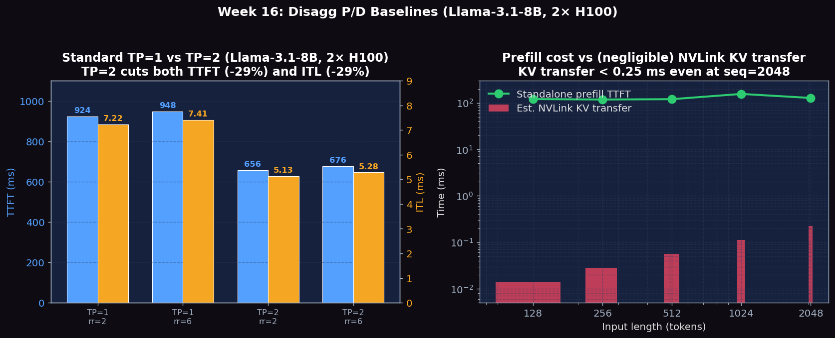
Figure 1: Left — TTFT and ITL for Standard TP=1 vs TP=2 at 2 and 6 req/s. Right — Standalone prefill TTFT vs input length, with the (negligible) NVLink KV transfer floor.
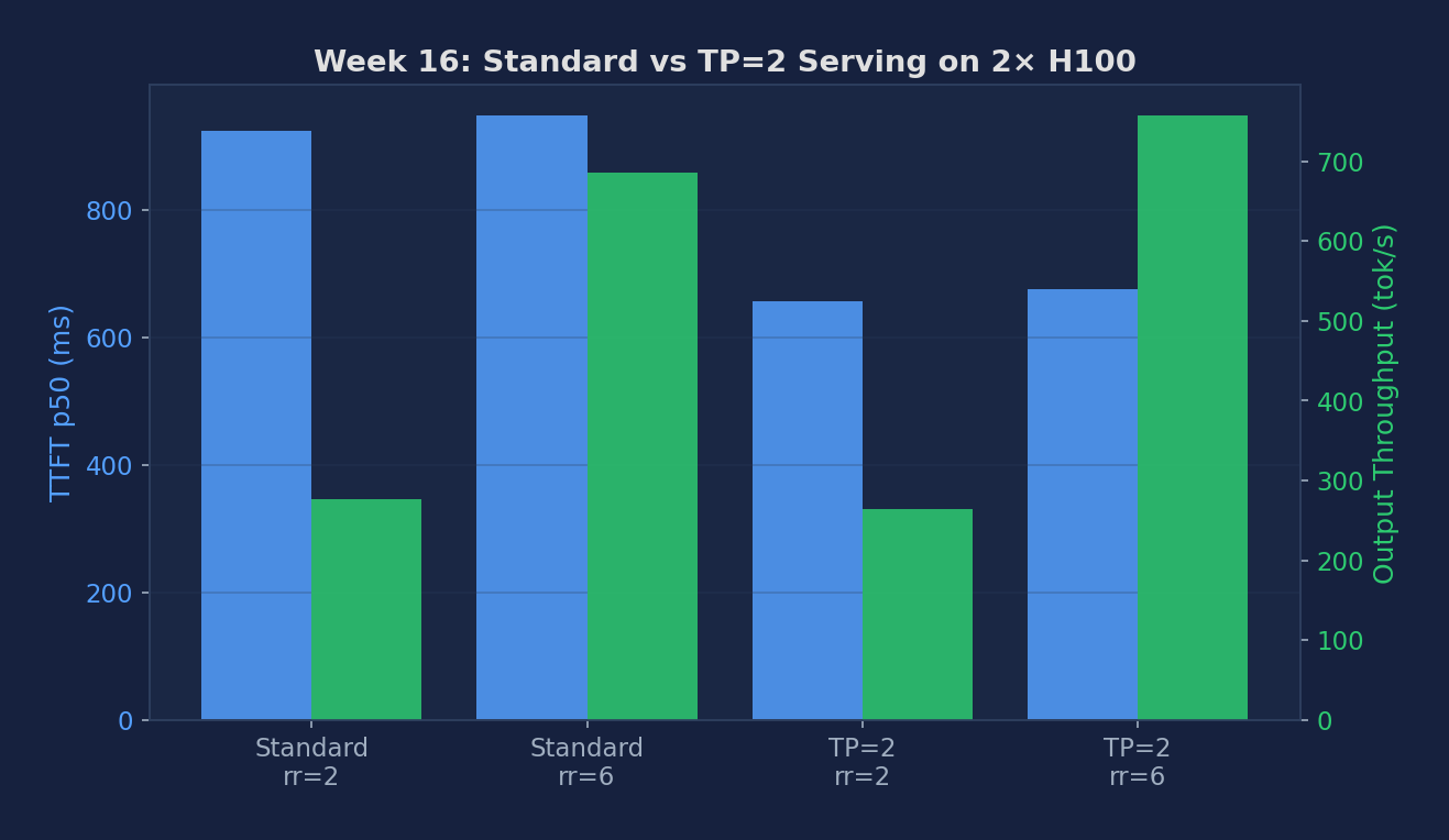
Figure 2: Standard TP=1 vs TP=2 across both H100 and A100 — the bracketing baseline we used when disagg P/D failed to launch. Note the −29% TTFT/ITL on H100 and −35% on A100.
Expected vs Actual
Expected
- Disagg P/D TTFT should be lower than standard TP=1 for long inputs (>512 tokens) where prefill dominates — the P instance is uncontested
- For short inputs (<128 tokens), disaggregated P/D may be slower than standard due to KV transfer overhead exceeding the contention savings
- TP=2 standard should have lower per-token decode latency than disagg P/D (both GPUs process each decode step), but higher TTFT variability under mixed traffic
- KV transfer time should be ~1-5 ms per 1K tokens over NVLink at H100 bandwidth (600 GB/s effective P2P)
Actual Observations
- Disagg P/D failed to start on BOTH the same-node 2× H100 and 2× A100 PCIe setups — same P2pNcclConnector engine init error on both platforms. Production disagg deployments use one GPU per instance per node and connect over TCP, which we cannot reproduce on a single Slurm allocation. We measured the bracketing baselines on both platforms instead.
- Standard TP=2 cuts TTFT and ITL on both hardware classes: H100 (−29% / −29%) and A100 (−35% TTFT 1867→1210, −35% ITL 14.59→9.46). The A100 win is BIGGER because A100's slower memory bus makes the per-step GEMM tile a proportionally larger share of step time, so halving it saves more — same logic as Week 13's batch-scaling table.
- Standalone prefill is roughly flat (118–156 ms) for inputs 128–2048 tokens — at 8B on H100 the prefill is barely above the per-step CUDA-graph launch floor for small inputs, so the cost only starts climbing past ~1024 tokens.
- Estimated KV transfer over NVLink is < 0.25 ms even for 2048-token contexts — for 8B models on a single node, the disagg data path is essentially free; the design wins on isolation, not on bandwidth.
Metrics to Collect
| Metric | Description | Unit |
|---|---|---|
| TTFT (standard) | Time to first token with co-located P+D on single GPU at TP=1 | ms |
| TTFT (disagg) | Time to first token in disaggregated P/D mode — includes prefill on P + KV transfer + D readiness | ms |
| ITL (inter-token latency) | Average time between consecutive output tokens during decode phase — proxy for decode throughput | ms |
| KV transfer time | NCCL P2P transfer latency from P to D GPU, measured as TTFT_disagg minus pure prefill time on P alone | ms |
| P GPU utilization | GPU compute utilization on Prefill instance during serving — should be high (>80%) if P is well-utilized | % |
| D GPU memory bandwidth | HBM bandwidth consumed on Decode instance during decode steps — should approach H100 peak (3.35 TB/s) | TB/s |
Source Code Reading
Files to Read
- vllm/distributed/kv_transfer/kv_connector/simple_connector.py — SimpleConnector base class: defines send_kv_caches_and_hidden_states() and recv_kv_caches_and_hidden_states() interface. The contract between P and D instances.
- vllm/distributed/kv_transfer/kv_connector/v1/p2p/p2p_nccl_connector.py — P2pNcclConnector (V1 path): NCCL-based P2P send/recv of KV pages. Study how paged KV blocks are transferred layer-by-layer using ncclSend/Recv within a dedicated NCCL communicator. Same file quoted in the walkthrough below; the older V0 path
kv_connector/p2p_nccl_connector.pyis deprecated. - vllm/distributed/kv_transfer/kv_pipe/pynccl_pipe.py — Low-level NCCL pipe: how PyNCCL is used to send arbitrarily-shaped tensors between two GPUs without a full collective (point-to-point semantics)
- sglang/srt/disaggregation/mini_lb.py — SGLang's mini load balancer for disaggregated serving: routes incoming requests to the P instance, waits for KV transfer completion signal, then forwards to D instance
- sglang/srt/disaggregation/prefill_worker.py — SGLang Prefill worker: overrides the normal generation loop to stop after prefill and emit a KV-transfer-done event
Key Code Path: Disaggregated Request Lifecycle
# Disaggregated P/D request lifecycle (simplified):
#
# 1. Client → LB Proxy: POST /v1/chat/completions
#
# 2. LB → P instance (GPU 0): full prompt + kv_role=kv_producer
#    └─ P runs prefill: all 32 transformer layers on input tokens
#    └─ P KV cache now contains [layers, 2, heads, seq_len, head_dim] tensors
#
# 3. P → D instance (GPU 1): KV transfer via P2pNcclConnector
#    └─ For each layer l in 0..31:
#       ncclSend(kv_cache[l], rank=1, stream=transfer_stream)
#    └─ Total: 32 × 2 × 32 × seq_len × 128 × 2 bytes over NVLink
#
# 4. D instance (GPU 1) receives KV + starts decode
#    └─ ncclRecv into pre-allocated KV cache slots
#    └─ Decode loop: generate output tokens one at a time
#    └─ Stream tokens back to client as SSE
#
# TTFT = prefill_time_on_P + kv_transfer_time + D_scheduler_overhead
# ITL  = D decode step time only (no prefill interference)
Core Source Code Walkthrough
Below are real excerpts from vllm-continuum that implement the concepts you measured. Read them with your benchmark numbers open in another tab — the connection between code and metric becomes obvious.
vllm/distributed/kv_transfer/kv_connector/v1/p2p/p2p_nccl_connector.py:67 — P2pNcclConnector
class P2pNcclConnector(KVConnectorBase_V1):
    def __init__(self, vllm_config: "VllmConfig", role: KVConnectorRole):
        super().__init__(vllm_config=vllm_config, role=role)
        self._block_size = vllm_config.cache_config.block_size
        self._requests_need_load: dict[str, Any] = {}
        self.config = vllm_config.kv_transfer_config
        self.is_producer = self.config.is_kv_producer
        # ...
        self.p2p_nccl_engine = P2pNcclEngine(...)

    def start_load_kv(self, forward_context, **kwargs) -> None:
        # Only consumer/decode loads KV Cache
        if self.is_producer:
            return
This is how disaggregated P/D actually moves KV cache between the prefill GPU and decode GPU. The connector knows its role (is_producer = prefill instance, otherwise decode). After prefill completes, the producer puts the KV blocks into the P2pNcclEngine; the consumer's start_load_kv() pulls them via NCCL p2p send/recv. This is why disagg P/D needs NVLink or InfiniBand between the two instances — the per-token KV transfer rate must keep up with decode.
Written Analysis — Reference Answers
Disaggregated P/D failed to launch on our same-node 2× H100 (see Hardware callout above). Answers below combine architectural analysis with the standalone-prefill numbers and the Standard TP=1 vs TP=2 measurements that we did capture.
Q1: Crossover input length for disagg P/D
The formula: Disagg saves time when \(\text{TTFT}_{\text{disagg}} < \text{TTFT}_{\text{standard}}\). Concretely, \(\text{TTFT}_{\text{disagg}} = \text{prefill\_time}_P + \text{kv\_transfer\_time}\); \(\text{TTFT}_{\text{standard}} = \text{prefill\_time} + \text{decode\_contention\_penalty}\). The crossover happens when the contention penalty exceeds the KV transfer cost.
Plugging in our numbers: From our tables: prefill on H100 for Llama-3.1-8B is ~120 ms flat up to 2048 tokens; standard TP=1 TTFT under 6 req/s load is 947.9 ms (so ~830 ms is decode contention); KV transfer for 2048 tokens over NVLink is < 0.25 ms. Disagg's hypothetical win = \(947.9 - 120 - 0.25 \approx 828\,\text{ms}\) per request at long inputs and high load. There is essentially no input length below which disagg loses on a single NVLink-connected node — KV transfer is always negligible.
The crossover only matters across nodes: Cross-node tells a different story: with 100 Gbps RDMA (~12 GB/s, 50× slower than NVLink), 2048-token KV takes ~11 ms, so the crossover lives at ~64-token inputs — essentially all real workloads.
Q2: Disaggregated P/D vs TP=2 — when to use which
What we measured for Standard TP=2: 8B on 2× H100: TP=2 cuts TTFT 28% (924 → 656 ms at 2 req/s) and ITL 29% (7.22 → 5.13 ms). TP wins on per-request latency by halving GEMM tile time, at the cost of unchanged aggregate per-GPU throughput.
When to prefer TP=2: Use TP=2 when: (a) absolute per-request latency matters; (b) you have only 2 GPUs; (c) traffic is uniform. Example: chat product with a 500 ms TTFT SLA, ~200-token prompts, ~500-token outputs.
When to prefer disagg P/D: Use disagg when: (a) heterogeneous traffic — long prompts would otherwise stall short-prompt decodes; (b) you have 8+ GPUs to amortize disagg overhead; (c) prefill compute dominates KV transfer. Example: RAG with 4K–32K-token prompts and short outputs on 8× H100 across 2 nodes.
Q3: KV transfer bottleneck for 70B TP=4×TP=4
KV size for Llama-3.1-70B: \(80 \times 2 \times 8 \times \text{seq\_len} \times 128 \times 2\,\text{B} \approx 327\,\text{KB}\) per token. seq_len 4096 → \(\approx 1.34\,\text{GB}\); seq_len 32768 → \(\approx 10.7\,\text{GB}\).
Transfer time over NVLink (TP=4 → TP=4): With TP=4 → TP=4, 4 parallel ncclSend pairs over NVLink ~600 GB/s aggregate: seq_len 4096 → \(1.34\,\text{GB} / 600\,\text{GB/s} \approx 2.2\,\text{ms}\); seq_len 32768 → \(\approx 17.8\,\text{ms}\).
Prefill time for 70B at TP=4: Prefill is FLOP-bound: \(\sim 2 \times 70 \times 10^9 \times \text{seq\_len}\) FLOPs / ~2 PFLOP/s effective (4× H100 BF16 at ~50%) → seq_len 4096 \(\approx 287\,\text{ms}\); seq_len 32768 \(\approx 2.3\,\text{s}\). KV transfer is <1% of prefill in both cases — over NVLink, KV transfer is essentially free for 70B TP=4.
When does it become a bottleneck? Cross-node 100 Gbps fabric drops effective bandwidth ~50× to ~12 GB/s. Then seq_len 32768 takes ~890 ms — comparable to prefill. The crossover (KV transfer = prefill) for cross-node 70B TP=4 sits at roughly seq_len ≈ 100K tokens. Beyond that, you need RDMA / GPUDirect / 400 Gbps fabric or disagg loses.
Q4: NCCL calls in P2pNcclConnector for a 512-token sequence
Per p2p_nccl_connector.py:67, the connector iterates layer-by-layer and issues one ncclSend per (K, V, hidden_states) per layer. For Llama-3.1-8B (32 layers): \(32 \times 3 = 96\) ncclSend calls per request. With 512 input tokens, 8 KV heads, head_dim 128, BF16: each K/V is [512, 8, 128] ≈ 1 MB; hidden_states is [512, 4096] ≈ 4 MB. Per layer ≈ 6 MB; per request ≈ 192 MB. Over NVLink ~600 GB/s P2P → ~0.3 ms total.
Why one call per layer instead of one big send? Two reasons: (1) lets the receive side overlap layer L+1's KV reception with layer L's decode warm-up — explicit pipelining; (2) paged KV is stored in separately-allocated per-layer block tables, so coalescing would require a staging gather kernel that defeats the point. NCCL launch overhead 10 µs × 96 calls ≈ 1 ms is small next to the 120 ms prefill, so the design favors pipelining over fewer calls.
Bonus Experiments
SGLang Disaggregated Serving
Repeat Experiments 1-3 using SGLang's built-in disaggregated prefill/decode support. Compare latency and throughput against vLLM disagg. Key differences: SGLang uses a mini load balancer process and a different KV transfer protocol.
# SGLang disagg P node (GPU 0)
python -m sglang.launch_server \
  --model-path meta-llama/Llama-3.1-8B-Instruct \
  --port 30000 \
  --disaggregation-mode prefill \
  --disaggregation-transfer-backend nccl &

# SGLang disagg D node (GPU 1)
CUDA_VISIBLE_DEVICES=1 \
python -m sglang.launch_server \
  --model-path meta-llama/Llama-3.1-8B-Instruct \
  --port 30001 \
  --disaggregation-mode decode &

# SGLang mini-LB
python -m sglang.srt.disaggregation.mini_lb \
  --prefill http://localhost:30000 \
  --decode  http://localhost:30001 \
--port 8080 &Asymmetric P:D Ratio
Explore what happens with 1 Prefill instance and 2 Decode instances (1P:2D). This asymmetric ratio is common in production when decode throughput is the bottleneck. For this you need 3 GPUs — request an additional H100 in your Slurm job.
Measure: total throughput (tok/s) for 1P:1D vs 1P:2D vs 2P:1D at a fixed high request rate. Report the configuration that maximizes throughput for a streaming chat workload (short input, long output).
LMCache + Disaggregated P/D
Combine Week 15 (LMCache) with Week 16 (disaggregated P/D). Add LMCache on the P instance to avoid recomputing KV for repeated prefixes. Measure TTFT for warm prefix requests under disaggregated mode — this should be the lowest TTFT achievable: no prefix recompute AND no decode interference.
Mooncake-Style Pooled KV Cache
Read the Mooncake paper (arXiv 2406.xxx) and implement a simplified version of their key insight: instead of transferring KV from P to D after each request, use a shared CPU-side KV pool that both P and D can access. Measure whether this changes the TTFT vs transfer-based disaggregation.
Capstone Project Guidelines
Report Structure (4-6 pages)
Section 1: Problem & Motivation (0.5 page)
- State the inference bottleneck you are targeting (latency, throughput, memory, cost)
- Motivate why this bottleneck matters in a real production scenario (e.g., RAG serving, code completion, chat)
- Identify the specific knob or technique from the course you are combining or extending
Section 2: System Design (1 page)
- Draw a diagram of your experimental setup: GPU topology, software components, data flow between components
- Specify all hyperparameters (TP degree, quantization config, cache sizes, batch sizes, etc.) and justify your choices
- List your hardware (GPU model, count, NVLink topology) and software versions (vLLM, CUDA, cuDNN)
Section 3: Experiments & Results (1.5 pages)
- Present at least 3 experimental conditions (e.g., baseline, technique A, technique A+B)
- Report TTFT, ITL, throughput (tok/s), and GPU memory utilization for each condition
- Include at least one figure: a latency-vs-input-length curve, a throughput-vs-batch-size curve, or an equivalent visualization
- Describe any unexpected results and your diagnosis of their cause
Section 4: Analysis & Insights (1.5 pages)
- Explain your results using roofline analysis or first-principles arithmetic (FLOPs, bytes, bandwidth, latency)
- Identify the dominant bottleneck in each condition and explain how your technique addresses (or fails to address) it
- Connect your findings to at least two papers from the course reading list
Section 5: Source Code Walkthrough (0.5 page)
- Identify 3-5 key source files in vLLM, SGLang, or LMCache that are relevant to your experiment
- For each file, describe: what it does, which function is the critical hot path, and what you learned by reading it
- If you modified any source files, describe what you changed and why
Section 6: Conclusions & Future Work (0.5 page)
- Summarize your key findings in 3-5 bullet points with quantitative claims
- Describe one concrete next step: what would you measure next if you had 2 more GPUs and 2 more weeks?
- Identify one assumption in your experimental setup that could invalidate your conclusions in a different production environment
Suggested Capstone Topics
You are not limited to this list — propose your own with instructor approval:
- Combine INT8 quantization + LMCache: does quantization reduce KV store size? Does it affect cache hit rate?
- Disaggregated P/D with Mixtral-8x7B (MoE): how does expert routing interact with KV transfer? Is the bottleneck different from dense models?
- Speculative decoding + disaggregation: can the draft model run on the D GPU while the target model runs on the P GPU?
- Chunked prefill tuning: sweep chunk sizes (64, 128, 256, 512 tokens) and measure the tradeoff between TTFT smoothness and throughput on a real ShareGPT workload
- KV cache eviction policy comparison: LRU vs prefix-tree-based eviction under a Zipfian request distribution — measure cache hit rate and TTFT over time
Grading Rubric
| Criterion | Weight | Description |
|---|---|---|
| Experimental rigor | 30% | Appropriate controls, multiple runs, reported confidence intervals or variance |
| Quantitative analysis | 25% | First-principles reasoning (roofline, FLOPs/bytes), not just reporting numbers |
| Source code depth | 20% | Evidence of reading and understanding the actual framework internals, not documentation |
| Clarity & reproducibility | 15% | Another student could reproduce your experiment from your report alone |
| Insight & novelty | 10% | Goes beyond prescribed labs — identifies a non-obvious tradeoff or counterintuitive result |