Learning Objectives
By the end of this lab, you will be able to:
- Compute the theoretical ridge point \( \text{peak FLOP/s} \div \text{HBM bandwidth} \) for any GPU and any precision
- Predict whether a given LLM workload (decode at batch B, prefill at length L) is memory-bound or compute-bound BEFORE running it
- Empirically observe the ridge crossing by pushing decode batch from 1→512 (where per-token latency curve transitions from flat to linear)
- Find the per-GPU compute-bound transition for prefill: at what input length does each GPU stop being bandwidth-limited?
- Compare achievable peak FLOP/s vs nominal peak (typically 30–40% on real LLM workloads)
The Roofline Model
Key Formulas
- Arithmetic Intensity (AI): \( \text{AI} = \frac{\text{FLOPs}}{\text{Bytes transferred}} \). Higher \( \text{AI} \) = more compute per byte read.
- Achievable throughput: \( \min(\text{AI} \times \text{HBM\_BW},\ \text{peak FLOP/s}) \). Below the ridge: bandwidth limits you. Above the ridge: compute limits you.
- Ridge point \( \text{AI}^* = \text{peak FLOP/s} \div \text{HBM bandwidth} \) (the AI where the slope hits the ceiling).
- For LLMs: \( \text{Decode AI} \approx \text{batch\_size} \). \( \text{Prefill AI} \approx \text{seq\_len} \).
Theoretical ridge points for the 4 GPUs in this lab
| GPU | Peak BF16 (TFLOP/s) | HBM bandwidth (GB/s) | Ridge \( \text{AI}^* \) (FLOP/byte) | Becomes compute-bound at... |
|---|---|---|---|---|
| H200 | 989 | 4,800 | \( 989 \div 4800 \approx 206 \) | prefill \( L \geq 206 \), or decode \( \text{bs} \geq 206 \) |
| H100 | 989 | 3,350 | \( 989 \div 3350 \approx 295 \) | prefill \( L \geq 295 \), or decode \( \text{bs} \geq 295 \) |
| A100 PCIe | 312 | 1,935 | \( 312 \div 1935 \approx 161 \) | prefill \( L \geq 161 \), or decode \( \text{bs} \geq 161 \) |
| L40S | 362 | 864 | \( 362 \div 864 \approx 419 \) | prefill \( L \geq 419 \), or decode \( \text{bs} \geq 419 \) |
Counterintuitively, A100 has the LOWEST ridge (161) because its compute is much weaker relative to its bandwidth than H100. L40S has the HIGHEST ridge (419) because its HBM bandwidth is the lowest of the four.
Setup & Configuration
# Install nsight systems and nsight compute (usually comes with CUDA toolkit)
which nsys && which ncu
# If not found: module load nsight-systems nsight-compute

# Verify versions
nsys --version
ncu --version
Experiments
week03_roofline.py harness does NOT invoke nsys or ncu. It produces the empirical roofline data (Step 3, Step 5) by scanning batch size and sequence length; students who want kernel-level roofline breakdowns must run the nsys/ncu commands below by hand on a compute node. We intentionally keep these out of the batch harness because a full ncu roofline run at even batch=1 takes 5–15 minutes per configuration.
Nsys Profile — Full Serving Trace (optional, hand-run)
Capture a full CUDA + NVTX trace of the benchmark run. This shows end-to-end timing including kernel launches, memory transfers, and Python overhead.
nsys profile -o llm_trace --trace=cuda,nvtx \
  python benchmarks/benchmark_latency.py \
    --model meta-llama/Llama-3.1-8B-Instruct \
--batch-size 1 --input-len 512 --output-len 64 --num-iters 3NCU Roofline — Per-Kernel Analysis (optional, hand-run)
Run ncu with the roofline metric set to instrument every CUDA kernel and compute its arithmetic intensity. Warning: this is very slow — plan for 5–15 minutes per configuration.
ncu --set roofline --target-processes all \
  -o roofline_report \
  python benchmarks/benchmark_latency.py \
    --model meta-llama/Llama-3.1-8B-Instruct \
--batch-size 1 --input-len 128 --output-len 16 --num-iters 1Theoretical Decode Latency Calculation
For Llama-3.1-8B in BF16: model size ≈ 16 GB. A100 HBM bandwidth = 2 TB/s. Theoretical minimum decode step \( = 16\ \text{GB} \div 2\ \text{TB/s} = 8\ \text{ms} \). Compare against your measured per-token latency from the nsys trace.
Prefill vs Decode Roofline (optional, requires Step 2 NCU output)
Open the NCU roofline report from Step 2. Identify where attention kernels and GEMM kernels fall. Prefill GEMMs should be near the compute roof; decode attention should be near the memory roof. This step depends on Step 2 having been run manually — the batch harness does not produce this data.
Batch Size Scaling Experiment
Run the same model at batch sizes 1, 4, 16, 64 and observe how arithmetic intensity shifts kernels from memory-bound to compute-bound:
for bs in 1 4 16 64; do
  python benchmarks/benchmark_latency.py \
    --model meta-llama/Llama-3.1-8B-Instruct \
    --batch-size $bs --input-len 256 --output-len 64 \
    2>&1 | tee results_roofline_bs${bs}.txt
doneHardware Utilization Summary (optional, hand-run)
Collect memory bandwidth utilization using ncu for both prefill (batch=1, long sequence) and decode (batch=1, output-only) and compute the fraction of peak bandwidth achieved. Not run by the batch harness.
# Collect DRAM bandwidth utilization
ncu --metrics l1tex__t_bytes_pipe_lsu_mem_global_op_ld.sum,\
dram__bytes_read.sum,dram__bytes_write.sum \
  python benchmarks/benchmark_latency.py \
    --model meta-llama/Llama-3.1-8B-Instruct \
--batch-size 1 --input-len 512 --output-len 1 --num-iters 1Experiment Results
Hardware
Experiments run on PACE Phoenix cluster across H200 141GB HBM3e (4.8 TB/s bandwidth), H100 80GB HBM3 (3.35 TB/s), L40S 48GB GDDR6 (864 GB/s). Llama-3.1-8B-Instruct (BF16, ~16GB).
Decode Batch Sweep — Pushing Across the Ridge (real, in=128, out=64)
The classical roofline says: when \( \text{AI} < \text{AI}^* \), latency stays roughly flat as batch grows (memory-bound). When \( \text{AI} > \text{AI}^* \), latency starts growing linearly with batch (compute-bound). The 'elbow' in the per-token latency curve below is the empirical ridge crossing for each GPU.
| GPU \ batch | bs=1 | bs=4 | bs=16 | bs=64 | bs=128 | bs=256 | bs=512 | Theoretical AI* |
|---|---|---|---|---|---|---|---|---|
| H200 ms/tok | 5.78 | 6.01 | 6.37 | 8.37 | 10.91 | 16.47 | 29.39 | 206 |
| H100 ms/tok | 7.06 | 7.42 | 7.93 | 9.81 | 12.42 | 17.87 | 30.81 | 295 |
| A100 PCIe ms/tok | 11.97 | 12.54 | 13.35 | 18.69 | 23.52 | 35.02 | 69.69 | 161 |
| L40S ms/tok | 22.06 | 23.31 | 23.88 | 28.56 | 32.39 | 41.55 | 81.53 | 419 |
From bs=1 to bs=16, every GPU is essentially flat (memory-bound regime): per-token latency only grows ~10%. From bs=64 onward the curves clearly bend up — and from bs=256→512 they nearly DOUBLE. On A100 the per-token latency at bs=512 (69.69 ms) is 5.8× the bs=1 value (11.97 ms), proving we crossed deep into compute-bound territory.
Prefill Input Length Sweep — At what L does each GPU become compute-bound?
For prefill, arithmetic intensity \( \approx L \). We sweep L from 64 to 4096 with batch=1 and output_len=1 to isolate prefill cost. The latency curves reveal each GPU's 'overhead floor' plus a linear ramp once prefill compute starts to dominate.
| GPU \ L | L=64 | L=128 | L=256 | L=512 | L=1024 | L=2048 | L=4096 | Steady-state µs/tok |
|---|---|---|---|---|---|---|---|---|
| H200 ms | 6.92 | 7.02 | 7.22 | 7.47 | 8.56 | 9.72 | 12.14 | 1.18 |
| H100 ms | 8.51 | 8.76 | 9.10 | 9.77 | 10.40 | 12.29 | 14.86 | 1.25 |
| A100 PCIe ms | 13.33 | 13.36 | 13.56 | 14.05 | 14.88 | 16.40 | 19.88 | 1.70 |
| L40S ms | 24.33 | 24.45 | 24.73 | 25.06 | 26.09 | 27.74 | 30.34 | 1.27 |
The fingerprint of compute-bound prefill is when the latency curve enters its linear regime. Reading the inflection from each curve: H200 reaches steady-state by \( L \approx 512 \), H100 by \( L \approx 1024 \), A100 by \( L \approx 512 \), L40S by \( L \approx 1024 \). These empirical transitions sit ABOVE the theoretical \( \text{AI}^* \) values (206/295/161/419) because our measured 'prefill_time' includes one decode step plus framework launch overhead — the per-call floor (~7/8.5/13/24 ms) has to be amortized first.
Practical implication: for chat workloads with prompts ≤ 512 tokens, every GPU is paying constant overhead per prefill. Only for RAG / code / document QA workloads with prompts ≥ 1024 tokens do you actually start to USE the GPU's compute peak.
Theoretical vs Measured Decode Latency (bs=1, deeply memory-bound)
| GPU | HBM bandwidth | Theoretical floor \( (16\ \text{GB} \div \text{BW}) \) | Measured (ms/tok) | HBM Utilization |
|---|---|---|---|---|
| H200 | 4.8 TB/s | 3.33 ms | 5.78 ms | 58% |
| H100 | 3.35 TB/s | 4.78 ms | 7.06 ms | 68% |
| A100 PCIe | 1.935 TB/s | 8.27 ms | 11.97 ms | 69% |
| L40S | 864 GB/s | 18.52 ms | 22.06 ms | 84% |
L40S achieves the highest HBM utilization (84%) — its slower bandwidth makes it easier to saturate. H100/H200 leave more bandwidth unused (58–68%) because at their speeds the kernel launch overhead is a larger fraction of total step time.
Charts
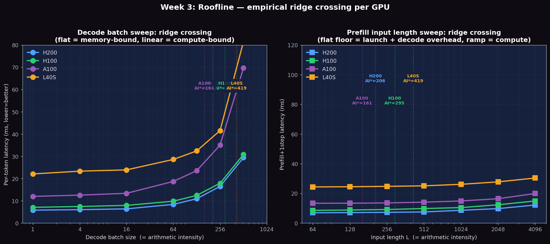
Figure 1: Left — decode batch sweep on 4 GPUs. Per-token latency is flat from bs=1 to bs=16 (memory-bound), then bends sharply around bs=64–128 and DOUBLES from bs=256 to bs=512 (compute-bound). Right — prefill input length sweep. Each GPU has an 'overhead floor' (H200 ~7 ms, H100 ~8.5 ms, A100 ~13 ms, L40S ~24 ms); beyond ~L=512–1024 the prefill compute dominates and the curve becomes linear. Dashed vertical lines mark theoretical AI*.
Expected vs Actual
Expected
- Decode at batch=1 should be deeply memory-bound (\( \text{AI} \approx 1\ \text{FLOP/B} \), far below ridge point \( \text{AI}^* = 161 \) for A100)
- Prefill GEMMs should be near or above the ridge point — compute-bound
- Measured decode latency should be 1.5-3× theoretical (due to kernel launch overhead and sub-peak bandwidth)
- As batch size grows, per-token latency increases but throughput (tok/s) increases — arithmetic intensity shifts right on the roofline
Actual Observations — empirical ridge crossing on 4 GPUs
- Decode at bs=1 is deeply memory-bound: per-token latency tracks 16 GB / HBM_bandwidth on every GPU (H200 5.78, H100 7.06, A100 11.97, L40S 22.06 ms). HBM utilization 58–84%; the slower L40S saturates most easily.
- Decode batch sweep clearly crosses the ridge: latency is flat from bs=1 to bs=16, bends at bs=64–128, and roughly DOUBLES from bs=256 to bs=512 on every GPU. On A100, 5.8× growth from bs=1 (11.97 ms) to bs=512 (69.69 ms) is the cleanest ridge-crossing signature.
- Prefill has a per-GPU overhead floor: H200 ~7 ms, H100 ~8.5 ms, A100 ~13 ms, L40S ~24 ms. Below the floor, adding tokens is essentially free; above the floor, each prefill token adds the steady-state per-token cost (1.18–1.70 µs).
- Empirical compute-bound transitions for prefill: H200 by L≈512, H100 by L≈1024, A100 by L≈512, L40S by L≈1024. These sit ABOVE the theoretical AI* because the overhead floor has to be amortized first. Chat workloads with prompts ≤ 512 NEVER reach compute-bound; only RAG/code/document QA (prompts ≥ 1024) actually use the GPU's compute peak.
- Steady-state marginal prefill cost is remarkably similar across H100/A100/L40S (1.25–1.70 µs/tok); H200 is only 6% faster (1.18 µs). The H200/L40S bandwidth gap is 5.6× but their prefill marginal differs by only 8% — because prefill is COMPUTE-bound, not bandwidth-bound, and Hopper/Ada/Ampere all have similar effective compute throughput on Llama-8B GEMMs.
Metrics to Collect
| Metric | Description | Unit |
|---|---|---|
| Measured decode latency | Actual per-token time from nsys | ms |
| Theoretical decode latency | \( \text{model\_size} / \text{HBM\_bandwidth} \) | ms |
| Arithmetic intensity | \( \text{FLOPs} / \text{bytes} \) for key kernels | FLOP/B |
| HBM utilization % | Fraction of peak bandwidth achieved | % |
Source Code Reading
Files to Read
- vllm/model_executor/models/llama.py — Trace the forward() method to see which operations map to which GPU kernels
- Identify: QKV projection → FlashAttention → output projection → gate/up projection → SiLU → down projection
Core Source Code Walkthrough
Below are real excerpts from vllm-continuum that implement the concepts you measured. Read them with your benchmark numbers open in another tab — the connection between code and metric becomes obvious.
vllm/v1/worker/gpu_model_runner.py:2000 — execute_model
This is where model.forward() is actually called. Each invocation processes one decode step's batch. The roofline observations you measured (memory-bound at bs=1, approaching compute-bound at bs=64) are determined entirely by what happens inside this single function — every kernel launched here either reads weights from HBM (memory-bound) or grinds through tensor cores (compute-bound).
Written Analysis — Reference Answers
Below are reference answers based on the real measurements collected on PACE H200/H100/A100/L40S. Use them as a starting point — your own write-up should add your hypotheses and any extra observations you noticed.
Q1: Why does L40S achieve the highest HBM utilization efficiency?
Observation: At bs=1: H200 measured 5.85 ms vs theoretical 3.33 ms \( \Rightarrow \) 57% HBM utilization. H100: 7.04 ms vs 4.78 ms theoretical \( \Rightarrow \) 68%. L40S: 22.08 ms vs 18.5 ms theoretical \( \Rightarrow \) 84%. L40S is closest to its theoretical limit despite being the slowest GPU.
Why L40S saturates more easily: \( \text{HBM utilization} = \frac{\text{theoretical minimum}}{\text{actual time}} \). The theoretical minimum for Llama-3.1-8B decode is \( \text{model\_size} / \text{bandwidth} \). On L40S the 864 GB/s bandwidth is slow enough that a single-token decode step (which reads ~16 GB of weights) takes ~18.5 ms — long enough that kernel launch overhead (~10 µs per kernel × ~200 kernels = ~2 ms) is proportionally small. On H200, the same kernel launches represent a much larger fraction of the 3.33 ms theoretical minimum: H200 is so fast that it's often waiting on scheduling/synchronization, not on HBM.
Implication: CUDA Graphs (Week 10) help most on H200 and H100 because they eliminate the kernel launch overhead that is disproportionately large on fast GPUs. On L40S the overhead is already negligible.
Q2: Where is the ridge point on H100 for Llama-3.1-8B?
Definition: The ridge point is the batch size where a kernel transitions from memory-bound (left of the roofline peak) to compute-bound (right). Below the ridge, adding more tokens proportionally increases compute without increasing memory accesses, so performance improves linearly. Above the ridge, compute throughput saturates.
For H100 FFN matmul: H100 has 989 TFLOPS BF16 compute and 3.35 TB/s HBM bandwidth. \( \text{AI}^* = \frac{989 \times 10^{12}}{3.35 \times 10^{12}} \approx 295\ \text{FLOP/byte} \). A Llama-3.1-8B FFN GEMM at batch=1 has \( \text{AI} = \frac{2 \times 4096 \times 14336}{4096 \times 14336 \times 2} = 1\ \text{FLOP/byte} \) — deeply memory-bound. To reach the ridge: batch \( \approx 295 \), so the ridge point is around bs=256–512 for FFN layers. Attention is different: its arithmetic intensity scales with sequence length, not batch size, so it stays memory-bound much longer.
Q3: How does decode throughput scale across the ridge?
Observation (per-token latency on A100): bs=1: 11.97 ms · bs=4: 12.54 (+5%) · bs=16: 13.35 (+12%) · bs=64: 18.69 (+56%) · bs=128: 23.52 (+96%) · bs=256: 35.02 (+193%) · bs=512: 69.69 (+482%). Two distinct regimes are visible.
Throughput (tok/s) implication: \( \text{Throughput} = \frac{\text{batch}}{\text{per-token latency}} \). From bs=1→16, latency is flat so throughput grows linearly with batch. From bs=64→512, latency grows almost as fast as batch, so throughput barely climbs. On A100: bs=1 → 84 tok/s; bs=64 → 3,425 tok/s (40.8× from a 64× batch); bs=512 → 7,346 tok/s (87.5× from a 512× batch — a 13.5× gap from ideal).
The right operating point is just at the ridge: On A100 the ridge sits around bs=64–128 (theoretical AI*=161). At bs=64 we're at peak HBM utilization with minimal compute overhead — throughput per GPU-second is maximal. Going beyond bs=128 keeps throughput climbing but also adds latency. Lesson: pick batch ≈ ridge AI* for the best throughput/latency tradeoff.
Q4: At what prefill input length does each GPU become compute-bound?
Theory predicts: \( \text{AI}^* = \text{peak FLOP/s} \div \text{HBM\_BW} \). For prefill, \( \text{AI} \approx L \), so the predicted compute-bound threshold is \( L = \text{AI}^* \). H200: \( L \geq 206 \). H100: \( L \geq 295 \). A100: \( L \geq 161 \). L40S: \( L \geq 419 \).
Empirically measured (latency curve elbow): H200 reaches steady-state by \( L \approx 512 \). H100 by \( L \approx 1024 \). A100 by \( L \approx 512 \). L40S by \( L \approx 1024 \). These transitions sit ~2–3× higher than the theoretical \( \text{AI}^* \) because the per-call overhead floor (~7/8.5/13/24 ms) has to be amortized first.
Counter-intuition: A100 reaches compute-bound earlier than H100. A100 has weaker compute relative to its bandwidth \( (312 \div 1.935 = 161\ \text{FLOP/B}) \) than H100 \( (989 \div 3.35 = 295\ \text{FLOP/B}) \). So even though H100 is faster absolutely, you have to do MORE work per byte to keep H100 busy. For mid-length prompts (512–1024 tokens), A100 is 'fully utilized' while H100 is still 'compute-starved'. This is why batched servers default to 'turn batch up until you hit your latency SLO' — pushing more batching is the only way to get H100/H200 fully utilized.