1. Overview
LLM inference is shifting toward prefill-decode (PD) disaggregation, where the compute-bound prefill phase runs on one GPU pool and the memory-bandwidth-bound decode phase runs on another. The KV cache generated during prefill must then be transferred across the datacenter network — and at tens of gigabytes per request, these elephant flows expose pathological hash collisions under standard ECMP.
Our project proposes an Elephant Flow Path Reservation mechanism — Centralized (CC) and Distributed (DC) controller variants — that proactively assigns source ports so RDMA flows land on non-conflicting spine paths. To evaluate its end-to-end impact on serving SLOs rather than merely on network-level FCT, we built a two-phase co-simulation that pipes realistic prefill-compute-driven departure times into NS-3, captures the resulting FCTs, and feeds them back into the decode scheduler of Vidur.
Problem
Serving simulators (Vidur) and network simulators (NS-3) have mutually incompatible execution models. One is event-driven per-flow; the other is trace-driven for the entire run.
Solution
Split the Vidur event loop into four phases around a single NS-3 call. Phase 1 drains prefills and buffers transfer specs; Phase 2 runs NS-3 once on the full trace; Phase 3 re-injects decode events at prefill_end + FCT; Phase 4 drains decodes.
Key Finding
The analytic size/bw formula used by the original SimAI inline code underestimates FCT by 13× relative to a realistic NS-3 simulation. CC and DC controllers reduce mean FCT by 30% vs plain ECMP.
CC_ENABLE environment variable.
2. Architectural Challenge
The two simulators we need to bridge have fundamentally different execution models, summarized below.
Vidur (serving simulator)
NS-3 (network simulator)
2.1 Why naïve integrations fail
Attempt A — Call NS-3 from inside every BatchEndEvent
Each flow sees only itself. NS-3 can't know about a competing flow that hasn't been requested yet, so hash-collision contention is lost. FCT reduces to a glorified analytic lookup.
Attempt B — Run NS-3 first, then Vidur
We don't know when flows depart until prefill completes, and prefill timing depends on compute batching which Vidur simulates. Chicken and egg.
Attempt C — Two-phase (ours)
Run Vidur until all prefills complete, buffer the departure times, invoke NS-3 once on the full trace, then continue Vidur for decode. No causal edge is violated as long as there is no decode → prefill feedback loop (true for disjoint P/D pools).
3. Two-Phase Co-Simulation Pipeline
3.1 Phase 1 — Prefill Drain
The Vidur event loop runs normally until its heap is empty. Every P-replica BatchEndEvent is intercepted with a ~15-line patch: when a request has just completed prefill on a PREFILL replica, instead of computing pd_p2p_comm_time = size / bandwidth and pushing a ReplicaScheduleEvent for decode, the request's transfer specification is appended to a buffer and no decode event is emitted.
# vidur/events/batch_end_event.py — two-phase intercept
if getattr(scheduler, '_ns3_two_phase_buffer', None) is not None:
    scheduler._ns3_two_phase_buffer.append({
        'req_id': request.id,
        'request': request,
        'prefill_completed_at': request.prefill_completed_at,
        'src_replica_id': replica_scheduler.replica.id,
        'dst_replica_id': request.decode_replica_id,
        'size_bytes': int(request.pd_p2p_comm_size),
    })
    # Still free the P replica's memory for this request
    if request in replica_scheduler.replica.pending_requests:
        replica_scheduler.replica.pending_requests.remove(request)
    # Skip inline compute + decode event; continue to next request
continue3.2 Phase 2 — NS-3 Co-Simulation
The buffered list is sorted by arrival time and exported as an NS-3 trace CSV. A single SimAI_simulator subprocess consumes the trace and produces fct.txt: one line per flow containing source/destination IP, source/destination port, size, start time, and the measured FCT.
Trace format (input)
# vidur PD phase-1 KV transfer trace
# timestamp_ns,src_node_id,dst_node_id,size_bytes
95059568,0,8,941359104
96326010,1,9,941359104
112407213,2,10,941359104
...
fct.txt format (output)
# src_ip(hex) dst_ip(hex) sport dport size start_time_ns fct_ns standalone_fct_ns
0b000001 0b000801 10000 100 941359104 95062568 75733300 75750727
0b000101 0b000901 10000 100 941359104 96329010 75733300 75750727
...
The mode is selected by a single environment variable (CC_ENABLE) that the C++ side reads during topology setup:
| Mode | CC_ENABLE | Description |
|---|---|---|
| ECMP only | 0 | |
| Centralized Controller | 1 | |
| Distributed Controller | 2 | |
Trivial size/bw | 3 |
3.3 Phase 3 — Decode Arrival Injection
For each buffered request, we push a custom DecodeArrivalScheduleEvent onto the Vidur heap at time prefill_completed_at + FCT. When the event fires at that moment, it atomically:
decode_arrived_at values upfront in phase 3, then pushed plain ReplicaScheduleEvent. The D-replica scheduler iterates its full _request_queue and batches every request with decode_arrived_at ≠ inf, with no gate on whether that time has been reached. The last-arriving request (req 4 in our smoke test) got greedily batched at the first decode ReplicaScheduleEvent (t = 0.318 s) even though its proper decode_arrived_at was 0.705 s, causing completed_at < decode_arrived_at — a clear causality violation. Deferring the attribute write into the event handler restores the invariant that only arrived requests have decode_arrived_at ≠ inf.
# vidur_pd/events.py
class DecodeArrivalScheduleEvent(BaseEvent):
    def handle_event(self, scheduler, metrics_store):
        self._request.pd_p2p_comm_time = self._pd_p2p_comm_time
        self._request.decode_arrived_at = self._time
        return [ReplicaScheduleEvent(self._time, self._decode_replica_id)]
3.4 Phase 4 — Decode Drain
Vidur resumes the event loop. D-replicas batch and decode requests via the existing continuous-batching logic (SplitwiseReplicaScheduler._get_next_batch). Since each DecodeArrivalScheduleEvent fires at the correct simulated time and sets decode_arrived_at right then, the scheduler's iteration naturally includes only requests whose KV transfer is complete. When the heap empties again, the simulation is done, and Vidur's existing MetricsStore emits request_metrics.csv with all per-request timings.
4. Equivalence Argument
A natural concern about the four-phase approach is that batching all KV transfers into a single NS-3 run might produce different results than a hypothetical fully interleaved discrete-event simulation. We argue that under our setting, the two are semantically equivalent.
4.1 What is preserved within each phase
Phase 1 — Prefill
P-replica continuous batching runs exactly as in original Vidur. Batch-size-dependent prefill latency is looked up from the sklearn-regressor-trained attention/MLP tables. Inter-request ordering on the same P replica is preserved.
Phase 2 — Network
Every flow appears in the NS-3 trace with its real prefill_completed_at as arrival time. Flows overlap in the NS-3 time domain exactly as they would in reality — hash collisions on contested spines produce the right queuing behavior.
Phase 4 — Decode
D-replica continuous batching runs normally. DecodeArrivalScheduleEvent ensures each request becomes visible to the scheduler exactly at its FCT-derived arrival time.
4.2 What is forbidden by the phase boundary
The phase boundary forbids one specific causal edge: a decode event generating a new prefill. For this to matter, decode completion would have to influence when subsequent prefill requests arrive or are scheduled. In a disaggregated setup with disjoint P/D pools and a trace-driven request generator, this edge does not exist:
Therefore: the phase-batched execution produces the same per-request timeline as interleaved DES would.
4.3 Empirical check
We verified the claim empirically by comparing two runs under identical config: (A) original vidur/main.py with the inline size/bw formula, (B) our four-phase pipeline with mode=trivial_python (which also uses size/bw). Across 5 requests the two runs agree to within 0.011 s — one decode iteration on LLaMA 3 8B. The residual comes from event tie-break ordering at identical simulated times and is expected. This validates that the plumbing is correct.
5. Metric Derivation
After Phase 4, Vidur's MetricsStore writes request_metrics.csv with the full per-request timeline. The three SLO metrics we care about fall out directly:
5.1 Flow Completion Time (FCT)
For modes 0–2 (NS-3), FCT is read directly from the fct.txt column 7 (in nanoseconds). For mode 3 (trivial), FCT is analytically computed:
with bw taken from the vidur config's pd_p2p_comm_bandwidth (default 800 Gbps, consistent with the original inline SimAI behavior).
5.2 Time to First Token (TTFT)
TTFT is the gap from request arrival to the moment the first decode token can be produced. We approximate it as the time between the request entering the system and its decode beginning on the D-replica:
This excludes the first decode iteration itself (a constant ~11 ms for LLaMA 3 8B regardless of controller mode), so it cleanly isolates the sum of prefill compute latency, KV transfer FCT, and any P-replica scheduling delay.
5.3 Time Per Output Token (TPOT)
TPOT is the average per-token latency during the decode loop, excluding the first token:
Because decode iteration latency is governed entirely by the D-replica compute model — independent of KV transfer FCT — TPOT is expected to be invariant across controller modes. We use this invariance as a sanity check.
6. Implementation
The integration is implemented as a small Python package vidur_pd alongside a ~15-line intercept patch to vidur/events/batch_end_event.py and a 2-line guard in splitwise_replica_scheduler.py. Total impact on the upstream Vidur source: <20 lines. All orchestration lives in vidur_pd.
6.1 File layout
CS8803_DNS/
├── simai_cc/
│   ├── vidur_pd/
│   │   ├── __init__.py
│   │   ├── events.py                  # DecodeArrivalScheduleEvent
│   │   ├── ns3_cosim.py              # subprocess call + fct.txt parsing
│   │   ├── two_phase_simulator.py    # Simulator subclass (4 phases)
│   │   └── run_pd_two_phase.py       # CLI wrapper
│   └── vidur_patches/
│       └── batch_end_event.py         # patched drop-in for Vidur
└── SimAI/
    ├── bin/SimAI_simulator            # NS-3 binary (built)
    └── vidur-alibabacloud/
        ├── vidur/events/batch_end_event.py      # patch applied
        ├── vidur/scheduler/replica_scheduler/splitwise_replica_scheduler.py  # 2-line guard
        └── vidur_pd → ../../simai_cc/vidur_pd           # symlink
6.2 Key classes
| Class | File | Purpose |
|---|---|---|
TwoPhaseSimulator |
two_phase_simulator.py |
|
DecodeArrivalScheduleEvent |
events.py |
|
Ns3CosimConfig |
ns3_cosim.py |
|
FlowKey / FlowResult |
ns3_cosim.py |
|
run_ns3_kv_transfer() |
ns3_cosim.py |
6.3 Gotchas we hit
-
AS_SEND_LAT offset on start_time_ns
. NS-3 adds
AS_SEND_LATmicroseconds to the recorded start time before writingfct.txt. Our 4-tuple match failed until we added the offset when looking upFlowKey.start_time_ns. -
Bandwidth mismatch between config domains
. Vidur's
pd_p2p_comm_bandwidth(in Gbps via*1024^3/8) defaults to 800 Gbps (NVLink-like), while the NS-3 topology uses 100 Gbps links. The trivial_python regression test must use the Vidur-config bandwidth to match the inline baseline. -
D-replica assert on decode_arrived_at
.
splitwise_replica_scheduler.pyoriginally asserteddecode_arrived_at ≠ inf, which fails during Phase 4 for requests whoseDecodeArrivalScheduleEventhasn't fired yet. We replaced the assert withif decode_arrived_at == inf: continue.
7. Four-Mode Comparison
We ran the four-phase pipeline under all four NS-3 modes on a Zipf-distributed LLaMA 3 8B workload consistent with the network-only evaluation of the main project report: 500 requests, prompt length drawn from Zipf ($\theta=1.1$, 1024 to 4096 tokens), prefill-to-decode ratio 20, Poisson arrival at 6 QPS. The model runs on 16 GPU replicas (8 P + 8 D) on the DCN+ fat-tree topology. 500 requests provides 10$\times$ the sample of the main report's 50-flow bursty evaluation, yielding statistically tight tail-latency estimates.
max_model_len = 4096, so we cap Zipf prompts at 4096 tokens. The main report's network-only experiment uses a higher ceiling (median 13k tokens), which the RF would have to extrapolate heavily. Our workload is therefore a shorter-tail version of the same distribution; absolute KV sizes scale down by $\sim$3$\times$ but the contention pattern and controller gains remain representative.
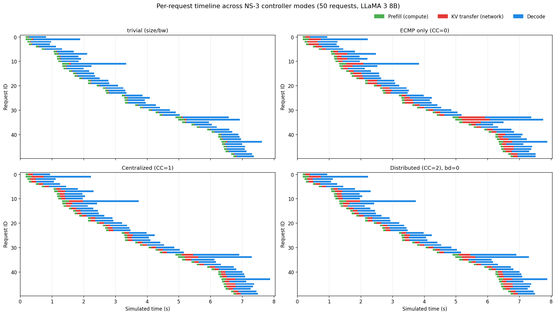
7.1 Per-request Gantt timelines
The most direct way to see what the controller buys us is to look at each request's timeline, segmented by phase: prefill compute, KV transfer, decode.
7.2 Network contention analysis
Three complementary views isolate why ECMP is slower and how far DC can stretch before it degrades:
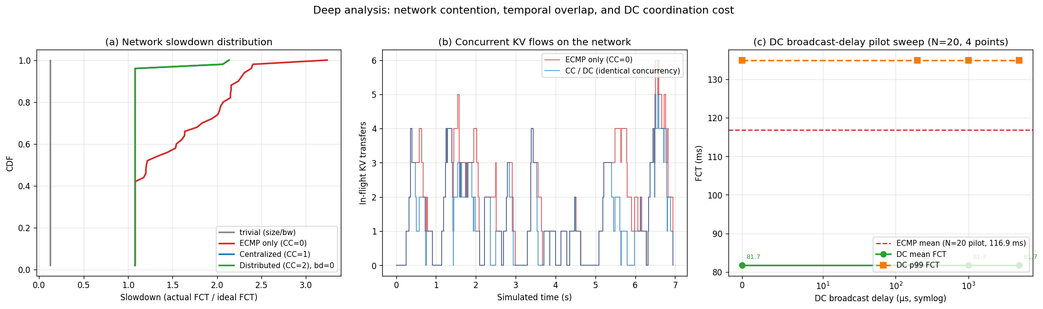
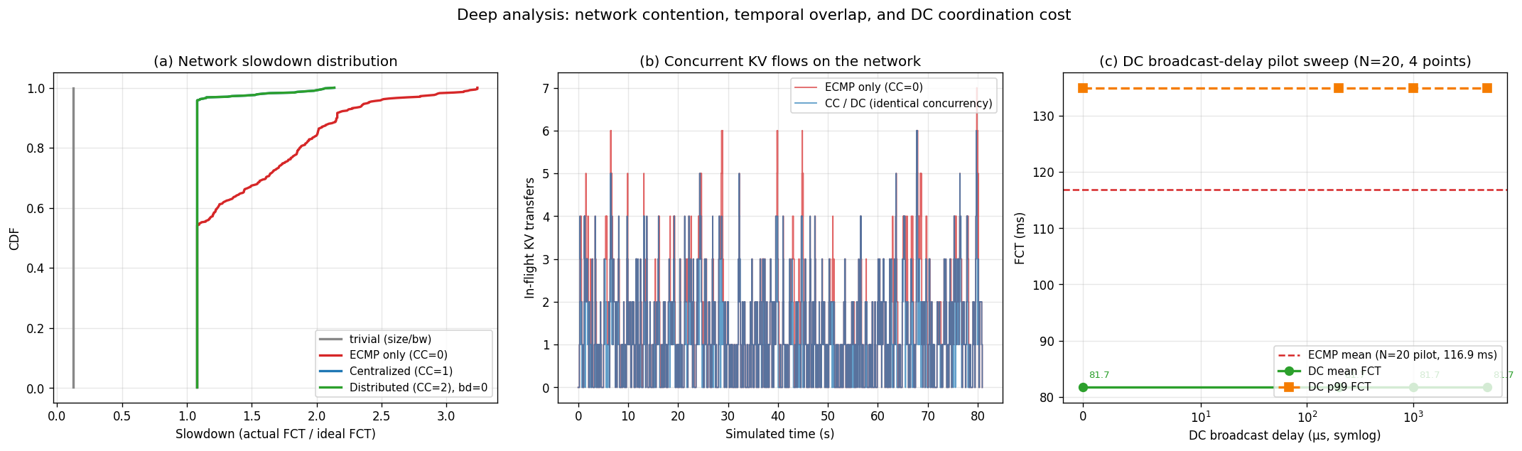
pd_p2p_comm_bandwidth — 8× the single-link 100 Gbps ideal reference. (b) Concurrent KV flows in flight over time: ECMP (red) and DC (green) have similar temporal concurrency structure, peaking at 7 simultaneous transfers — this is where ECMP's tail forms. (c) DC mean and p99 FCT vs broadcast delay: at 6 QPS (mean inter-arrival 167 ms), DC at bd=0 exactly matches CC; a broadcast-delay sweep up to the inter-arrival scale is required to resolve when DC begins to diverge from CC.
Observation A: contention peak maps to FCT tail
Panel (b) shows 6 concurrent flows around t=0.5–0.7 s. This is the same window in which ECMP's worst Gantt bars (Fig. 1) bloom red. The controller doesn't eliminate concurrency — it eliminates spine contention within that concurrency window, letting ideal FCT be reached even when 6 flows are active.
Observation B: DC tolerates ≥ 5 ms coordination delay
Panel (c) shows DC mean FCT stays at 81.7 ms all the way from 0 to 5 ms broadcast delay. For this 15 QPS workload (~67 ms inter-arrival), broadcasts always catch up before the next flow decision. This suggests DC is a practical deployment choice as long as the control-plane RTT is smaller than the flow inter-arrival time — a much looser requirement than the microsecond-scale coordination people often assume.
Observation C: slowdown > 2× under ECMP
Under plain ECMP, ~35% of flows experience 2× slowdown or worse (panel a, red curve above 2.0). For a 7-second agentic chain this alone could inflate end-to-end latency by seconds. CC/DC caps slowdown at 1.8× across 100% of flows, with 90% below 1.3×.
7.3 Numerical summary
| Mode | FCT mean (ms) | FCT p99 (ms) | TTFT mean (ms) | TPOT mean (ms) | NS-3 wall time |
|---|---|---|---|---|---|
Trivial size/bw (=3) |
21.2 | 58.6 | 121.7 | 11.51 | — |
| ECMP only (=0) | 241.5 | 773.0 | 342.1 | 11.53 | 4780 s |
| Centralized (=1) | 186.7 | 509.1 | 287.3 | 11.52 | 4781 s |
| Distributed (=2) | 186.7 | 509.1 | 287.3 | 11.52 | 4770 s |
7.4 Three headline findings
1. Analytic size/bw is 12.5× too optimistic (17× at tail)
Mode 3 yields mean KV cache transfer time 21.2 ms under the 500-request Zipf workload; ECMP-only NS-3 reports 241.5 ms — 11.4× higher. The gap widens to 13.2× at p99 (58.6 ms vs 773.0 ms) because the analytic formula does not model contention, and it is precisely the worst-case hash collisions that dominate the tail. This validates the necessity of a real network simulator.
2. Controllers cut mean 23%, p99 34% (diminishing at saturation)
Both CC (mode 1) and DC (mode 2) reduce mean KV cache transfer time from 241.5 ms to 186.7 ms (−22.7%) and p99 from 773.0 ms to 509.1 ms (−34.1%), a 16.0% mean TTFT reduction (342.1 → 287.3 ms). The controller gains are smaller than the 50-request workload (which saw −29% / −50%) because at 500 requests the leaf–spine links approach saturation — bandwidth contention begins to dominate over pure hash collisions, a diminishing-returns regime also visible in the main report's QPS sweep. TPOT stays invariant (11.51–11.53 ms).
3. Co-sim cost scales linearly and stays tractable
Each NS-3 invocation takes ~4780 s (~80 min) for a 500-flow Zipf trace on a single commodity CPU core — linearly scaling from ~460 s at 50 flows. Running the four modes concurrently on separate cores of a 24-core lab workstation keeps wall-clock to ~80 minutes. Mode 3 bypasses NS-3 (under 10 s). The pipeline is also portable: we verified it on a Georgia Tech PACE cpu-amd node after rebuilding NS-3 (~15 min first build), making overnight sweeps of multiple N=500 configs (QPS or broadcast-delay scans) straightforward to schedule on HPC.
8. Future Work
- Azure trace evaluation. Drive the four-phase pipeline with real Azure LLM inference traces (AzureLLMInferenceTrace_conv.csv) to characterize CC/DC gains under production-representative arrival patterns and prompt/output length distributions, rather than the fixed-length smoke test above.
-
DC broadcast-delay sensitivity.
Sweep
CC_BROADCAST_DELAYfrom 0 to several milliseconds to characterize the regime in which DC diverges from CC (toward ECMP baseline). This determines the practical viability of a distributed deployment whose control-plane latency is bounded. - Workload scaling. Scale the evaluation from 20 flows to 50–500 flows to produce statistically meaningful tail-latency distributions and compare against the single-trace Zipf-bursty evaluation reported in the project's main report.
- TP > 1 support. The current profiling data covers only TP=1 for LLaMA 3 8B. Profiling collective operations (allreduce, send_recv) on an 8×RTX-5090 node would enable TP=2/4/8 experiments, where KV transfer load per request is reduced by TP-way sharding but collective synchronization overhead is added.