Part I · What exists
Three layers, three different optimization objects
The first six sections establish the workload and then compare stored attention state, low-level computation, and request scheduling. The aim is not a list of systems: it is a map of what each layer can observe, what it can safely change, and where its assumptions stop.
1. Why agent workloads stress serving infrastructure
The workload comes first because every later mechanism is a response to the same physical pattern: long shared prompts, many dependent model calls, and pauses whose duration is set by tools or external state. This section defines that pattern before comparing solutions.
A multi-agent system, abbreviated MAS, coordinates several model-driven roles or agents to complete one application-level task. Attention is the mechanism by which a token reads prior tokens. Each model call has a prefill phase, the initial computation that reads the prompt, and a decode phase, the repeated computation that emits new tokens. During both phases the model stores key and value attention tensors for prior tokens; this stored attention state is the KV cache. Reusing an exact KV prefix avoids repeating prefill.
Two latency terms recur throughout the page. Time to first token, or TTFT, measures the delay from request arrival until the first generated token and is especially sensitive to prompt prefill. Job completion time, or JCT, measures the whole workflow. P95 and P99 are the delays below which 95% and 99% of observations fall. A service-level objective, or SLO, is a promised latency or completion bound; goodput counts only work that completes within that bound, rather than all raw throughput.
The three cards below establish the workload scale through reusable-token share, session activity, and per-program prompt growth.
SMetric’s production traces establish that agent traffic contains more repeated state than ordinary chat. The number describes potential sharing, not realized cache hits; generic serving can still discard the useful state.
TraceLab shows that open-ended coding agents are not short request chains. They repeatedly alternate between model inference and external actions, so cache lifetime and the next consumer cannot be reduced to one fixed batch.
Continuum’s trace makes prompt growth concrete. Its mean tool time is 925 ms with a 3,550 ms standard deviation, so the gap between dependent calls is both useful for movement and difficult to predict from a mean.
Pythia, a production study of an agent-serving platform (arXiv 2604.25899), reports that agentic workflows account for more than 80% of requests on the studied platform, while more than 40% of those workflows obtain zero or limited cache hits; single-minute request spikes for one model reach 50.3% above its baseline load. These values jointly mean that high reuse potential is not enough: the runtime must know which retained state is likely to matter, and it must remain correct when that knowledge is incomplete.
Read the four-step strip from left to right as the lifecycle of one turn, from its shared prefix through transcript growth and an external gap to the conditional continuation.
System instructions, tools, and examples recur across calls.
Each turn adds messages and tool results, increasing prefill cost.
A tool or human suspends the next model call for an uncertain interval.
The result can choose another agent, retry, terminate, or create a new branch.
The infrastructure problem is therefore not one-dimensional. InferCept measures 37–40% of forward time as avoidable interception waste in paused workloads, while the cache studies below show that numerical reuse can become incorrect when context changes. The next three sections separate these concerns by layer: state construction, attention computation, and workflow scheduling.

2. KV-cache layer: reuse, repair, and communication
The workload evidence points first to stored attention state: repeated prefixes make reuse valuable, while changing context makes reuse unsafe. This section compares what each KV mechanism reuses, what it repairs, and the workload assumption that limits it.
Four terms recur in this section: radix tree, checkpoint, non-prefix reuse, and eviction. Exact prefix reuse is the simple case: the same tokens occupy the same positions behind the same causal history, so the stored state is already correct. A radix tree is a prefix tree that stores a shared token sequence once and branches only where requests differ. A checkpoint is a saved set of model weights and configuration. Non-prefix reuse is harder because rotary positional encoding, or RoPE, rotates attention coordinates according to token position, and because a cached token may not have attended to the context that now precedes it. Repositioning can repair coordinates; it cannot by itself reconstruct missing conditioning. Eviction means removing retained state to free cache capacity.
The rebuilt diagram below separates three objects that are often called KV reuse even though they require different proofs. It is followed by a mechanism table so that the visual categories are tied to concrete systems rather than treated as an informal taxonomy.
A low-rank representation approximates a large correction with a small number of basis directions. It can reduce work, but it is exact only when the discarded directions carry no required information.
Color notation. Blue = $p$ (shared prefix); orange = $t_A$ / $t$; purple = $t_B$; green = recomputed tokens or $p_B$; gold = $\ell$ (trained link); gray = $q$ / unique content.
The layer axis is elided in these three overview panels; §2.3 restores it in every system-level grid.
Notation preview. $KV(x \mid y)$ names the layerwise state of $x$ under preceding string $y$. Panel A reuses exact state. Panel B starts from independently cached $t_A$ and $t_B$ and seeks the estimate $\hat{KV}(t_B \mid t_A)$. Panel C transfers A's output $t$ from prompt $p_A$ toward the receiver-conditioned estimate $\hat{KV}(t \mid p_B)$. The complete symbol register and proof-style transformations appear in §2.3.
This comparison is scenario-first: read the “Built for (scenario)” column before the mechanism columns. The remaining columns explain what state is reused, how damage is repaired or state is composed, what signal drives the decision, whether training or profiling is needed, and where the design stops helping; scroll horizontally to see the full table.
| System | Built for (scenario) | State reused | Repair or composition | Decision signal | Training or profiling | Primary shortfall |
|---|---|---|---|---|---|---|
| CacheBlend Scenario B |
A RAG server assembles several retrieved documents into one prompt. Each document’s KV cache was precomputed separately, so the assembled prompt is not a simple prefix hit; CacheBlend repairs the stitched cache instead of prefilling the whole prompt again. | It reuses KV tensors that were precomputed independently for each retrieved document chunk, including chunks placed away from the prompt prefix. | It realigns RoPE positions and recomputes roughly 10–20% of high-deviation tokens layer by layer so the selected tokens recover missing cross-chunk conditioning. | For the realized query-and-chunk assembly, it compares newly computed and loaded KV state across layers to keep the high-deviation tokens in the repair set. | It requires no model training; token selection runs online, while the loading controller uses offline profiles of recomputation and storage latency. | Because damage depends on the realized query, chunks, and order, the system must repeat selection and repair for every new assembly. |
| EPIC / LegoLink Scenario B |
A serving platform repeatedly builds prompts from immutable documents or few-shot examples that appear in different orders and positions. EPIC compiles each chunk once, and LegoLink repairs a fixed boundary region when the chunks are linked for a request. | It reuses independently compiled, position-independent KV caches for immutable chunks whose local positions begin at zero. | For each non-first chunk, LegoLink recomputes at most its first 32 sink tokens, meaning initial tokens that tend to absorb disproportionate attention. | It chooses the repair set solely from each static chunk boundary, without inspecting the current query or measuring token-specific damage. | It needs no weight training or request-specific profiling because the boundary rule and its token limit are fixed before serving. | Because its repair is query-insensitive and confined to chunk beginnings, it can miss assembly-specific damage farther inside a chunk. |
| KVLink Scenario B |
A RAG or QA service wants to encode a large document library once and later combine only the documents retrieved for each query. KVLink reconnects those independently cached documents without re-encoding their full text. | It reuses each retrieved document’s context-free KV cache, which was precomputed without the other documents or the current query. | It re-encodes keys for their global positions, then uses trained link tokens under a custom attention mask to restore information flow among independently encoded documents. | It has no query-aware damage detector; its learned link-token bottleneck and fixed mask determine how every document exchanges information. | It jointly trains the modified checkpoint and link tokens for 6,000 steps on eight H100 GPUs. | The fine-tuned checkpoint, added link-token interface, and custom mask form a coupled serving package, so a different backbone needs another training path. |
| KVCOMM Scenario C |
A multi-agent pipeline uses one checkpoint, but planner, coder, and judge prompts place shared text behind different role-specific prefixes. KVCOMM adapts that text’s cache to each receiver instead of making every agent prefill the overlap again. | It reuses full KV tensors for shared text under the same checkpoint, even when another agent originally created them behind a different prefix. | It removes the original RoPE rotation, applies the rotation for the receiver’s positions, and adds context-dependent Key and Value offsets interpolated from online anchors. | It first filters anchors for compatible sequence length, then uses embedding distance to weight nearby anchors; the entropy of those weights decides whether the match is reliable enough for reuse. | It requires no weight update or offline profiling; fallback prefills populate and update an online anchor pool. | It cannot safely reuse state when a new prefix lacks a nearby compatible anchor and must fall back to dense prefill; its own sweep also shows reasoning accuracy decreasing as reuse becomes more aggressive. |
| KVComm Outside · readout |
A stable sender–receiver pair needs to pass rich context without making the sender decode a natural-language message at every handoff. KVComm transmits selected sender KV layers and lets the receiver attend to that internal state directly. | It transmits all context tokens’ Key and Value pairs from a calibrated, potentially non-contiguous subset of sender layers. | The receiver concatenates the transmitted pairs into the corresponding attention layers during prefill and decoding; it does not repair or recompute the unshared sender layers. | Offline calibration ranks layers by query-to-context attention mass plus a Gaussian middle-layer prior, then fixes the selected set for the model pair and dataset. | It requires no weight training, but each sender–receiver pair and dataset needs its own layer calibration. | Direct layer matching assumes identical models or fine-tunes of the same base architecture, so unseen pairs and changing agent graphs are unsupported without new calibration. |
| Cache-to-Cache Outside · cross-model |
A specialist model from one family must hand its semantic understanding to a receiver from another family, even though their tokenizers and layer spaces differ. Cache-to-Cache learns a direct cache channel instead of serializing the intermediate result as text. | The receiver consumes per-layer semantic KV state produced by a sender from another model family alongside its own cache. | Trained per-layer fusers align the models, project and residually combine both caches, and apply learned head weights and layer gates. | Input-conditioned head weights and learned layer gates determine which transferred semantics enter the receiver. | Both LLMs remain frozen, but the fuser must be trained separately for every model pair. | Pairwise training does not extend automatically to new models, and an inaccurate sender can transfer incorrect semantics rather than merely numerical cache error. |
| DroidSpeak Outside · checkpoint |
A workflow switches among fine-tuned models derived from the same base model, and several specialists must process the same long context. DroidSpeak hands off prefix KV and recomputes only the layers profiled as critical for that model pair. | It reuses prefix KV tensors between fine-tuned models that have the same architecture and tensor shapes. | It recomputes the profiled groups of critical layers for the receiver and reuses the remaining sender layers. | Offline profiling measures which layer groups preserve output quality for their recomputation cost, producing a quality–cost frontier for each source–target pair. | It requires $O(L^2)$ pairwise profiling, where $L$ is the number of layers; the reported setup took about three hours for each model pair. | A new model pair or model drift can invalidate the pair-specific profile and require profiling again. |
| RelayCaching Scenario C |
An upstream agent decodes a plan or answer that a downstream agent then inserts into its own prompt. RelayCaching converts the upstream decode-time state into downstream prefill state instead of re-encoding the generated text in full. | It reuses the upstream agent’s decode-time KV tensors and a boundary hidden state produced while generating the output. | It relocates cached positions with RoPE and selectively recomputes high-risk tokens within a profiled range of layers. | An offline profile identifies the layer range likely to need correction, while online KV deviation and accumulated-attention influence identify the tokens to repair. | It requires no weight training, but it needs calibration data for the intended sender–receiver route. | It assumes identical model architectures and a stable calibrated route, so heterogeneous models or distribution shifts can require full prefill or recalibration. |
| LatentMAS Outside · latent |
An ordered planner–worker–judge workflow does not need human-readable text between intermediate agents; only the final role must answer the user. LatentMAS keeps the intermediate exchange in latent working memory instead of repeatedly decoding and re-encoding text. | It carries forward complete layer-wise KV working memory containing both the input context and the agents’ generated latent thoughts. | A one-time linear alignment operator maps each last-layer hidden state back into the input embedding space, while complete layer-wise KV is transferred by exact concatenation. | It uses no token or layer selector; the workflow’s ordered predecessor relation determines which complete memory is handed to each successor. | It needs no fine-tuning for the mapping because the alignment operator is computed once and then reused. | It changes the communication contract and relies on ordered, same-shaped KV handoffs, so it is not a transparent solution for arbitrary concurrent or cross-family composition. |
| Kamera Scenario B |
A multimodal agent repeatedly revisits, reorders, evicts, or recalls the same video frames, UI screenshots, or document pages as its context window and multi-hop reasoning evolve. Kamera reuses those chunks without re-encoding the full multimodal context. | It reuses a position-free canonical KV cache for each multimodal chunk together with a compact, antecedent-conditioned patch. | It applies exact RoPE re-rotation to move a chunk to its target position, then adds a low-rank feature patch that restores lost cross-chunk conditioning. | One conditioned compile-time forward measures the contextual KV delta, and its dominant low-rank directions define the patch instead of a query-time token selector. | It is training-free, but constructing each patch requires one conditioned forward at compile time. | A changed antecedent requires a fresh patch, while fixed-prefix or dense-text cases with no cross-chunk conditioning gap gain little from the mechanism. |
| ProphetKV Scenario B |
A latency-sensitive RAG request has a limited recomputation budget, and only some tokens in the assembled documents matter to the user’s final query. ProphetKV directs that budget toward query-relevant tokens rather than generally salient ones. | It reuses position-independent KV caches produced for retrieved document chunks in isolation and inserted away from the prompt prefix. | It fuses query-to-context scores across layers and recomputes one fixed, query-selected token set through every layer. | Attention from the final query tokens to the assembled document context determines which tokens enter the repair set. | It requires no fine-tuning or offline profiling, but it performs its lightweight selection pass for each assembled request at serving time. | It cannot select a repair set until the final query and all retrieved chunks have been assembled, so earlier dynamic stages receive no repair decision. |
2.1 Repair accuracy is part of the systems result
Two text-quality metrics appear next. F1 balances precision, the share of selected items that are correct, and recall, the share of relevant items found. ROUGE-L measures longest-common-subsequence overlap with a reference. A decrease means the reused state changed answer quality.
CacheBlend’s reported 2.2–3.3× TTFT reduction is paired with a quality loss of 0.01–0.03 F1 / ROUGE-L points when 10–20% of tokens are recomputed; full reuse without repair loses roughly 0.1–0.2 F1 or 0.03–0.25 ROUGE-L in its evaluated tasks. EPIC reports up to 8× TTFT and 7× throughput, but its direct CacheBlend comparison is up to 3× and allows at most 7% accuracy loss. The contrast is architectural: CacheBlend spends work to locate damage in the realized assembly, while EPIC assumes the first few tokens of each later chunk carry the important boundary error, meaning the missing conditioning introduced where chunks meet.
KVLink reports up to 96% TTFT reduction after training, yet naive concatenation loses as much as 35% relative question answering (QA) quality and the learned method requires 6,000 training steps on eight H100 GPUs. KVCOMM is training-free and reaches a reported 7.82× five-agent prefill speedup, but its own threshold sweep moves from 34.3% reuse with 83.1% accuracy to 98.2% reuse with 78.8% accuracy. These paired values establish a recurring rule: a larger numerical reuse ratio is not evidence of a better agent system unless the receiving route’s quality is measured.
The next rebuilt diagram isolates position variance. It matters here because an agent response cached at one offset may be embedded later behind a different role prompt or transcript, even when its token text is unchanged.
2.2 State of the art by reuse regime
The badge under each system name makes its scenario contract explicit, because these methods are not interchangeable implementations of one API: compatibility, training, and fallback obligations differ. Scenario A still has no table row: exact prefix reuse needs no repair, so radix caching, Hydragen, and RelayAttention are discussed in §3.
Panel B today — repairing $KV(t_A)\|KV(t_B)$ toward $\hat{KV}(t_B \mid t_A)$
Panel B contains five successive ways to repair or redefine independently prefilled chunks. CacheBlend starts with deviation-selected token recomputation for the realized assembly. EPIC / LegoLink replaces online selection with a fixed first-$k$ attention-sink boundary. ProphetKV makes the budget query-aware: the terminal $q$ chooses one token set from all-layer attention. KVLink changes the checkpoint and mask contract, using trained link tokens $\ell$ to reconnect context-free chunks. Kamera moves the correction into feature space, storing a low-rank patch after exact key relocation.

The current B-regime verdict is no longer just “which tokens should be recomputed.” At an equal 20% recompute budget, ProphetKV prices cross-chunk binding at 100/73.5/50.5 for ProphetKV/CacheBlend/EPIC. Kamera’s measurements further show that the damage has low-rank structure in feature space and is concentrated in deeper layers; deepest-half-only patching remains an optional, model-dependent variant, but the result shows why token-granular recomputation can be the wrong axis. For MAS, B-regime SoTA therefore means assembling agent contexts from independently compiled spans and choosing the repair unit—tokens, trained links, or features—against receiver quality rather than maximizing reuse alone.
Panel C today — moving $KV(t \mid p_A)$ toward $\hat{KV}(t \mid p_B)$
RelayCaching derives a correction for each realized relay: it relocates the upstream decode state, then selectively replaces tokens through a profiled middle-layer range. Its received-attention influence selector outperforms deviation-only selection, 84.8 versus 79.7. KVCOMM instead amortizes correction through remembered anchors: it re-rotates keys, interpolates receiver-specific offsets from similar eligible messages, and falls back to dense prefill plus a new anchor when dynamic topology produces an uncovered prefix. Both pursue the same receiver-conditioned target, but the open question is the correction source—derived per relay, remembered in anchors, or learned—not one universal reuse operator.
Outside the panels
Section 2.3 keeps four off-diagram treatments explicit. KVComm is a direct-read channel over selected sender layers and does not reconstruct textual KV. DroidSpeak changes checkpoints and recomputes a pair-profiled layer interval. Cache-to-Cache learns cross-model semantic fusion while preserving the receiver’s own cache. LatentMAS transports all-layer latent working memory without an intermediate text $t$. Because each changes an object or compatibility variable held fixed by panels B and C, these four contracts do not compete in B/C SoTA.
2.3 How each system transforms its state
The eleven diagrams now isolate one mechanism each. Scenario-B methods repair or redefine independently cached chunks; scenario-C methods transport a runtime message between prefixes; the remaining four systems change the communication object or compatibility contract, so they are stated without forcing them into scenarios A–C.
Notation used in the transformations
- $KV(x)$
- the layerwise key–value state of token string $x$ when prefilled alone
- $KV(x \mid y)$
- the state of $x$ computed with string $y$ before it
- $\hat{KV}$
- an approximate KV state produced without full recomputation
- $t_A,t_B$
- two independently cached chunks
- $p_A,p_B$
- the prompts of agents A and B
- $t$
- a string produced by agent A
- $q$
- the query or request-unique suffix
- $\ell$
- trained link tokens
- $l,L$
- a layer index and the layer count
- $S_l$
- the token set recomputed at layer $l$
- $\Delta,\hat{\Delta}$
- a positional or contextual offset and its estimate
- $W,W'$
- two model checkpoints, usually sender and receiver
- $L^*$
- a selected layer subset
- $F_\theta$
- a trained cross-model projector or fuser
- $\pi(l)$
- the sender layer aligned to receiver layer $l$
CacheBlendarXiv:2405.16444
Scenario BGrid convention: columns are token positions and rows are transformer layers, shallow at top and deep at bottom; blue = $p$, orange = $t_A$ / $t$, purple = $t_B$, gray = $q$, green marks recomputation, patching, or reading, and gold marks trained elements; batch, KV-head, and hidden dimensions are omitted by research-diagram convention.
Insight. Once positions are corrected, sparse cross-chunk attention makes cache error highly nonuniform: roughly 10–15% of tokens have much larger KV deviation, and repairing higher-deviation tokens reduces attention deviation most (§4.3, Insight 1; Figs. 6–7). Those high-deviation rankings are also strongly correlated between adjacent layers (§4.3, Insight 2; Fig. 8). Together, these observations justify seeding selection with a full first-layer pass and gradually filtering a roughly 10–20% repair set across later layers instead of recomputing every token (Fig. 9).
Where: $l$ indexes the layer and $i$ the token; $t_A,t_B$ are the independently cached chunks and $\|$ concatenates them; $KV_{l,i}(t_B)$ is token $i$'s independently cached pre-relocation state at layer $l$; $C_{l,i}$ is that entry after positional offset $\Delta$ is applied by key-only $\mathrm{RoPE}^{K}$; $KV^{\mathrm{new}}_{l,i}$ is the fresh check state and $\Delta_{KV}$ is its state-distance from $C_{l,i}$; $d_l(i)$ is that deviation score; the FIRST layer is fully recomputed to seed the selection ($r_1$ slightly above the target ratio, e.g. 15%); each deeper layer re-ranks only within the previous set, so $S_{l+1} \subseteq S_l$ with $r_{l+1} \le r_l$ (gradual filtering, justified by the cross-layer correlation of high-deviation tokens); $\hat C_l$ is the current assembled hybrid cache; $\operatorname{Recomp}_{l,i}$ recomputes one selected entry against that cache; and $\hat{KV}_{l,i}$ is the repaired approximation.
CacheBlend mechanism. It repositions every cached key and recomputes the tokens estimated to be most damaged by the realized assembly. A full early check seeds nested candidates, while the released implementation ranks squared value deviation; about 10–20% of tokens are selected. After the check layer, recomputation uses the evolving hybrid cache, not an otherwise fully exact cache.
EPIC / LegoLinkarXiv:2410.15332
Scenario BInsight. Independent compilation resets every chunk's position IDs to zero, and the naively assembled attention map develops a repeated sink at each document beginning that diverts attention from relevant evidence (§4.1, Fig. 4). CacheBlend's dynamic 15% repair set frequently includes those same initial tokens, while EPIC's ablation shows that recomputing only a few chunk-initial tokens recovers most accuracy (§4.1; §5.3, Fig. 6). The stable location of the defect therefore supports a static, query-independent boundary prior with $k \le 32$, rather than rediscovering repair tokens for every request (§1; §4.2).
Where: $t_1,\ldots,t_c$ are the $c$ independently compiled chunks; $j$ ranges from 2 through $c$ in the union and, from 1 through $c$, identifies token $i$'s containing chunk in the reuse branch; $\operatorname{First}_{k}(t_j)$ returns the first $k$ positions of chunk $t_j$; $k$ is the fixed boundary width from 0 through 32; the union forms the all-layer sink set $S$; $l$ and $i$ index layer and token; $\|$ concatenates chunks; $\hat C_l$ is the current hybrid cache; $\operatorname{Recomp}_{l,i}$ recomputes a selected entry; $KV_{l,i}(t_j)$ is the independently cached entry retained outside $S$; and $\hat{KV}_{l,i}$ is the composed approximation.
EPIC / LegoLink. LegoLink repairs the local attention sinks at the beginning of every later chunk with one query-independent boundary set shared by all layers. The uncached query is computed normally and attends to every causally visible position. The paper compiles each chunk from position 0 and does not specify a global RoPE relocation in the proposed sketch; entries outside the boundary remain cached.
ProphetKVarXiv:2602.02579
Scenario BEach retrieved chunk ($t_A$, $t_B$; more in general) is cached independently from position 0 (top); at serving time the chunks are assembled with visible boundaries (bottom), and the QUERY attends over every chunk in a light all-layer pass — the resulting scores $v_i$ rank tokens from $t_A$ and $t_B$ TOGETHER, so the repair set $S$ is chosen globally across chunks, not per chunk.
Insight. Static boundary heuristics and KV- or hidden-state-deviation criteria reconstruct global attention without asking which evidence the current query needs; under a fixed budget, globally active but query-irrelevant tokens can displace query-critical ones—the crowding-out effect (§3.1, Figs. 2–3). The terminal query's own attention strongly overlaps the context tokens later read during decoding across model families, while its attention over the imperfect assembled cache is observable without full prefill (§3.2, Fig. 4; §4.2). This inexpensive relevance proxy supports one lightweight all-layer scoring pass and a global cross-chunk top-$p$ repair set, directing the budget toward correctness for the present query (§4.3; Appendix A, Algorithm 1).
Where: $q$ is the assembled request query and $Q_s$ its query-token positions; $t_1,\ldots,t_c$ are all cached chunks, with $C$ cached context tokens in total; $u,i,l$ index query token, context token, and layer; $Q_s^{(l)}$ is the lightweight query-pass representation, while $K_{1:C}^{\prime(l)}$ is the assembled imprecise/precomputed context-key cache used to measure $A^{\prime(l)}$—not oracle full-prefill attention; $d_k$ is key width; $\bar a_i$ uniformly fuses each layer's query-to-context column score; $T_p$ is one global top-$p$ token set over every chunk and is reused at all $L$ layers; $KV^0(t_j)$ is chunk $j$'s independently compiled cache and $\Delta_j$ its runtime relocation; $\hat C_l$ is the evolving hybrid cache; and $\operatorname{Recomp}$ fully recomputes selected tokens through the layer stack. Query tokens are computed normally at every layer to obtain the scores but are not repair-budget tokens.
ProphetKV mechanism. The final query pays for a lightweight all-layer scoring pass, after which only the context tokens most relevant to that query are recomputed. The evaluated default assigns 20% of the context to the shared repair set. Consequently, the selection becomes available only after the query and retrieved chunks have been assembled.
KVLinkarXiv:2502.16002
Scenario BInsight. Even after global RoPE positions are corrected, independently encoded document caches still lack the cross-document dependencies that later documents would have acquired from earlier ones (§§2.1–2.3). Table 1 makes the distinction concrete: the position-corrected PromptCache baseline scores 28.9% on Llama-3.1-8B NQ versus 71.3% for the original model, whereas KVLink5 reaches 72.5% (§3.1, Table 1). This evidence motivates a narrow, trained cross-document interface through which newly computed state can carry preceding-document context while the expensive document encodings remain reusable (Fig. 2).
Where: $i$ indexes a token and $x_i$ is its pre-projection representation; $W_K,W_V$ are the key and value projections; $C_i$ is the canonical position-free pair, while $R_{\operatorname{pos}(i)}$ restores its runtime key position and leaves values unchanged; $t_A,t_B$ are independently compiled documents and $KV^0$ denotes their context-free state from position 0; $\ell_A,\ell_B$ are freshly run blocks of $K$ trained link tokens appended to each document (the paper evaluates $K=1$ and $K=5$); each link block attends its current document plus all preceding documents and links under fine-tuned mask $M_{\mathrm{link}}$; $q$ is then processed with ordinary causal attention over the logical sequence shown; $\mid$ records conditioning and $\|$ its five state segments. The implementation may pack link blocks for its forward, but the equation preserves their logical after-document positions.
KVLink contract. Under the custom mask, document tokens keep their local conditioning while the trained link tokens attend across the current and preceding documents and links. The method therefore changes both checkpoint and mask contracts: it fine-tunes the model and link embeddings so that the link-token interface carries cross-document information. It does not claim to reconstruct the ordinary receiver-conditioned cache of the second chunk.
KameraarXiv:2606.23581
Scenario BInsight. Independently cached chunks preserve what a later query can read because attention over separate key sets admits an exact state merge, but they erase the conditioning that each chunk would have absorbed from earlier chunks; this asymmetry leaves single-hop retrieval intact while breaking cross-chunk binding (§§1–2). In the paper's multimodal workloads, that missing term is spread across tokens—an oracle selector needs about half of them—yet its effect on the output distribution saturates near rank 32 in feature space and grows sharply with depth (§4, Fig. 3). Sparse token repair therefore targets the wrong axis for the studied multimodal streams, motivating a deep feature-space correction.
Where: $l$ indexes a layer and $t_B$ is the context-free cached chunk; $p_0,p_1$ are its compile and target start positions and $\delta$ their displacement; $R_l^K(\delta)$ deterministically relocates only the RoPE-bearing key channel (the full key for GQA/MHA or $k_{pe}$ for MLA), leaving values/content channels unchanged; $C_l(\delta)$ is therefore the relocated canonical base; one conditioned compile of $\mathrm{prefix}\cdot t_A\cdot t_B$ at target positions supplies the exact $t_B$ state used to fit contextual deficit $\Delta_l^{\mathrm{ctx}}$; $\operatorname{SVD}_r$ retains rank $r$ per layer and relevant K/V channel or head, with singular values absorbed into $U$; and serving first relocates the base, then adds $U_{l,r}V_{l,r}^{\top}$ at every core layer without a forward pass. Deepest-half-only patching is an optional Appendix C.3 storage approximation, not the core operator.
Kamera patch. One conditioned compile-time forward measures the contextual residual, and reuse adds its low-rank feature correction without token recomputation. Rank 16 is an evaluated operating point rather than a fixed rule: the paper reports a knee around ranks 8–16, a plateau near 32, and an additional rank-64 evaluation. Patching only the deepest half of the layers remains an optional, model-dependent variant rather than the core operator.
RelayCachingarXiv:2603.13289
Scenario CInsight. An upstream agent's reply reaches the next agent as text even though its decode-phase KV has already been computed, so downstream prefill repeats work on identical tokens solely because their prefix changed (§1, Fig. 1). Those decode caches remain globally close to full-prefill caches and their residual error is structured, but numerical deviation is not the same as importance: moderately deviated tokens can matter when later reply tokens repeatedly attend to them during upstream decoding (§§3.1–3.3; §4.3). On GSM8K, deviation-only selection attains 79.68% accuracy, adding attention-derived influence reaches 81.65%, and the suffix safeguard completes the method at 84.84% (Table 3), motivating influence-aware repair.
Where: $t$ is agent A's generated message and $p_A,p_B$ are sender and receiver prompts; $Z$ is A's decode cache after deterministic key-only RoPE relocation by $\Delta_{\mathrm{pos}}$; $j$ is a handed-off token and $H$ the attention-head count; $v^{\mathrm{reuse}}$ and $v^{\mathrm{full}}$ are the reused and all-token-recomputed value vectors compared at detector layer $L_{\mathrm{det}}$, so $d_j$ is measured cosine deviation rather than an assumed score; $a_{ulhj}$ is attention received by $j$ over decoding steps $u$, profiled layers $l$, and heads $h$, and $I_j$ is its influence sum; bars are tokenwise means and $\tau_d,\tau_I$ thresholds; $K_{\mathrm{suf}}$ is the suffix safeguard length (default 10); $\mathcal I_t$ is every message-token index; $\mathcal R$ first recomputes all tokens on $[L_{\mathrm{start}},L_{\mathrm{det}})$ from saved transition $h_A^{L_{\mathrm{start}}}$, then only union-selected $S$ on $[L_{\mathrm{det}},L_{\mathrm{end}}]$; outside $\mathcal R$, relocated cache $Z$ is reused.
RelayCaching operator. The operator selectively replaces state rather than adding a patch. Every handed-off token is recomputed from the lower interval boundary through detector layer $L_{\mathrm{det}}$; only the selected set continues through the remaining profiled middle layers, while entries outside the interval reuse $Z$. Adding received-attention influence and the suffix safeguard raises the reported accuracy from 79.68% for deviation-only selection to 84.84% for the full selector.
KVCOMMarXiv:2510.12872
Scenario CInsight. The same shared text can acquire vastly different contextual KV offsets under different role prefixes, while an unaligned RoPE shift can be orders of magnitude larger still; raw reuse or one static correction is therefore unreliable (§1, Fig. 1; §3.1). After positional alignment, however, embedding-near samples exhibit correspondingly near changes in their KV offsets across prefixes (§3.2, Proposition 2; Fig. 4(c–d)). This locally gated regularity—not global smoothness over arbitrary prefixes—makes observed, agent-specific offsets useful as online anchors for recurring, segmentable prompt templates (§§3.3–3.4, Fig. 3).
Where: $\phi_{m,i}$ is agent $m$'s runtime placeholder and $\mathbf p_{m,i}$ its following fixed-prefix segment; $\mathcal A$ is that placeholder's anchor pool, $\psi$ an anchor, and $\mathcal A_\phi$ the length-compatible subset at least as long as $\phi$; $\mathcal L,h$ denote token length and message embedding; $w$ is embedding-distance similarity; $\gamma$ is the shareability threshold and $\mathcal P_{\mathrm{anchor}}$ means fallback/new-anchor creation—reuse proceeds only when every prompt placeholder makes it false. The paper calls $\mathcal H$ entropy but its displayed Eq. (5) omits the conventional leading minus; the equation above preserves that printed sign. $R^K$ deterministically de-rotates/re-rotates each base key to its target position and never rotates values; only contextual key/value residual pairs $(\Delta\mathbf k,\Delta\mathbf v)^\phi$ and $(\Delta\mathbf k,\Delta\mathbf v)^{\mathbf p}$ are similarity-interpolated. Each anchor stores those distinct placeholder and following-prefix K/V offsets, and the same $w$ updates them separately before concatenation.
KVCOMM interpolation. The method re-rotates keys and interpolates a receiver-route correction from similar messages rather than from nearby prompts. If any placeholder fails the length-compatibility or relative-entropy shareability test, the route falls back to dense prefill, measures the message and neighboring-prefix offsets, and records a new anchor. The approximation is therefore supported only where the evolving anchor bank covers the realized route.
KVCommarXiv:2510.03346
Outside · readoutInsight. Natural-language handoff expends multiple decoding steps and loses information through sampling, but a last-hidden-state shortcut also trades away savings: late-layer information concentrates in the final token, whereas passing all token states helps mainly at early layers (§2.2, Figs. 2–3). KV usefulness is instead nonuniform across depth; intermediate layers and layers with larger receiver-query-to-sender-context attention transfer best (§3.2; §4.3, Fig. 6; §4.5, Fig. 8). That selectivity licenses direct, untransformed KV sharing through a calibrated subset on aligned architectures; 30%, 50%, and 70% are tested budgets, and 70% is generally Skyline-comparable (§4.2, Table 1).
Where: $a^l_{hqc}$ is exact calibration attention at layer $l$ and head $h$, from receiver query token $q\in Q$ to sender-context token $c\in C$; $H$ is the head count and the paper averages over $H|Q|$—there is no extra $|C|$ divisor; $\hat S_a^l$ is that layer's sender-context attention mass and $S_a^l$ its across-layer MinMax normalization; $\alpha$ mixes this measured signal with a Gaussian depth prior centered at $\mu$ with spread $\sigma$; $L^*$ is the potentially non-contiguous top-$M$ index set, calibrated once for a sender–receiver model pair and dataset/task (one calibration sample in the experiments), with budgets 30%, 50%, or 70% of layers. At each same index $l\in L^*$, receiver queries read concatenated sender/receiver K/V; no arbitrary cross-layer pairing occurs.
KVComm (2510.03346). The receiver directly reads sender state at a calibrated 30%, 50%, or 70% of layers and uses only its own state elsewhere. It therefore creates a direct-read channel rather than reconstructing textual KV for the receiver. The selected layers are specific to the sender–receiver model pair and calibration dataset or task, so unseen pairs remain unsupported.
DroidSpeakarXiv:2411.02820
Outside · checkpointInsight. Because same-foundation model variants preserve similar understanding of a shared context, the authors hypothesized that most sender cache state should remain reusable even though full-cache reuse severely damages accuracy (§1; §3.2, Fig. 6). Their layer ablation confirmed nonuniform output sensitivity: across eight model pairs, only 11% of layers on average were individually critical, and the critical identities were largely stable across inputs for a given pair (§3.2, Insights 2–3; Figs. 7–8). That stable pair-specific sparsity makes offline profiling worthwhile; the recomputation span is contiguous not because the critical layers are, but because multiple reuse-to-recompute transitions require large E caches and propagate error (§4.1, Figs. 9–10).
Where: $W$ and $W'$ are sender and receiver checkpoints; $X=p\|t$ is the entire shared prefix/context tensor shown in the grid, not only transferred substring $t$; $l$ indexes a layer; $G^*=[a,b]$ is one contiguous interval selected from the pair-specific $O(L^2)$ profiled candidates and its quality/cost Pareto frontier for the runtime SLO; $E_a^W(X)$ is the sender's full-context transition E-cache injected once at boundary $a$; $\operatorname{Recomp}^{W'}_{a:l}$ means sequential receiver-weight execution from $a$ through $l$ seeded by that activation, rather than independently recomputing isolated layers; sender K/V for all tokens is reused outside $G^*$; and $\hat{KV}^{W'}$ remains an approximation to a full $W'$ prefill.
DroidSpeak transfer. Because the receiver's interval starts from a sender transition activation, the result remains an approximation to full prefill under the receiver checkpoint. DroidSpeak profiles every sender–receiver model pair, constructs a quality-versus-recomputed-layers Pareto frontier, and selects one contiguous interval for the runtime SLO. The reported 11% denotes individually sensitive layers rather than a universal recomputation budget.
Cache-to-CachearXiv:2510.03215
Outside · cross-modelInsight. Text is a low-bandwidth cross-model channel: it compresses high-dimensional internal state into ambiguous strings and adds sequential generation latency (§1, Fig. 2). The cache-enrichment oracle raises accuracy from 58.42% to 62.34% at the same cache length, while the transformation oracle shows raw source and target caches far apart in representation space but a learned map moving source state into the target space (§3.2, Table 1; Fig. 3). This supports the premise that model-specific coordinates can carry alignable contextual semantics; Table 8's 20.70 to 44.88 to 47.95 progression is projected replacement, then residual fusion, then layer gating, showing that receiver-state preservation and selective fusion—not projection alone—are essential (§4.4).
Where: $X$ is common input text, not a literally shared token sequence: frozen sharer $M_1$ and receiver $M_2$ tokenize it independently; $L_s,L_r$ are their layer counts; terminal alignment $\pi$ pairs final layers backward, so if the receiver is deeper its unmatched shallow layers retain receiver-only state; $\operatorname{TokAlign}_X$ aligns sender positions to receiver tokens by decoded-string coverage (including one-to-many matches); $F_{\theta,l}$ is the pair-specific residual fuser whose internals perform feature projection, feature fusion, input-aware head weighting, and a learned layer gate; the receiver's own prefetched base is always preserved by the outer plus; and both LLMs remain frozen while $\theta$ is trained.
Cache-to-Cache fusion. The trained fuser aligns tokens and layers, projects features, applies input-aware head weights, combines state residually, and uses learned per-layer gates while both LLMs remain frozen. C2C therefore preserves the receiver's own prefilled cache and adds selected sharer semantics rather than deriving receiver state from sharer KV alone. The ablation averages rise from 20.70 for projected replacement to 44.88 after residual fusion and 47.95 after gating, which attributes the gain to semantic complementarity.
LatentMASarXiv:2511.20639
Outside · latentInsight. Under the paper's Linear Representation Hypothesis, losslessly expressing an $m$-step latent trajectory requires $\Omega(d_hm/\log|\mathcal V|)$ text tokens, so discretization can either lose expressiveness or greatly lengthen the trajectory (§3.1, Theorem 3.1). A successor would then have to ingest that long textual trace, whereas KV already accumulates the predecessor's context and latent thoughts as working memory and can preserve them without re-encoding (§2; §3.2, Fig. 3; Theorem 3.3). This motivates keeping intermediate reasoning and handoff in latent space and verbalizing only at the final agent, avoiding the textual reconstruction problem rather than repairing it (§3.3, Theorem 3.4).
Where: $\mathcal M_A$ is agent A's all-layer latent working memory; $K$ and $V$ denote keys and values; subscripts $A,B$ identify source and receiver agents; the $\mathrm{cache}$ tag identifies stored layer state; $l$ indexes a transformer layer and $L$ is the layer count; $\equiv$ defines the transported object; the set-builder bar ranges that definition over every layer; $\leftarrow$ updates B's state; and $\|$ concatenates A's cached component before B's component at the same layer.
LatentMAS memory. The all-layer latent working memory itself becomes the message, so no textual intermediate or receiver-conditioned textual-KV approximation is formed. Its pseudo-inverse alignment maps an agent's last hidden state back to that same agent's next latent input; it is not a cross-agent cache repair. The handoff consequently assumes an ordered workflow and compatible transformer-layer shapes.


Layer conclusion. KV mechanisms focus on avoiding state reconstruction. Their common shortfall for dynamic MAS is not simply that a future graph is absent: compatibility is often tied to a realized query, a stable route, a model pair, or a trained checkpoint. Section 9 returns to the stricter correctness question when multiple predecessor contexts converge.
3. Kernel layer: compute shared attention once
The kernel layer begins after exact reusable state is known, but the five systems place that boundary differently. Hydragen and RelayAttention receive an explicit sharing contract; ChunkAttention discovers exact prefixes inside the active batch; FlashInfer composes caller-supplied sparse segments; SGLang discovers and retains prefixes across requests at runtime.


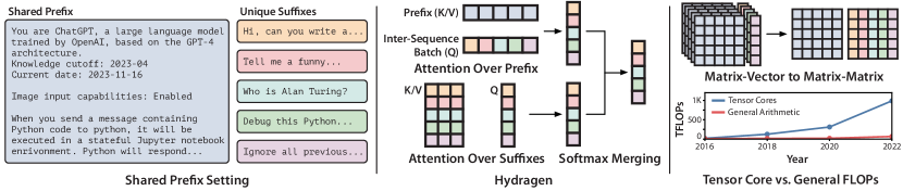
Four axes prevent unlike results from being conflated: where attention is decomposed, where the saving lands, what prefix identity must hold, and whether reuse requires a concurrent batch or can persist across time. LSE is the sufficient normalization state for exactly merging attention over disjoint visible key/value segments; the merge changes execution, not model semantics.
The central contrast is therefore not simply ‘prefix sharing.’ Hydragen changes the arithmetic shape from repeated matrix–vector work to an inter-sequence matrix–matrix operation; RelayAttention removes repeated off-chip reads for one fixed system prompt; ChunkAttention changes the active-batch traversal order; FlashInfer supplies a composable kernel algebra; RadixAttention changes runtime admission, retention, and scheduling.

The comparison matrix fixes the denominator for the detailed readings below. Kernel timing, decode-only throughput, end-to-end serving throughput, and runtime cache-hit rate answer different questions; every result is therefore paired with its operating regime.
| System | Decomposition point | Where the saving lands | Exact-prefix contract | Batch regime and evidence | Dynamic-MAS shortfall |
|---|---|---|---|---|---|
| Hydragen | caller-declared shared node versus request-specific suffixes | batched prefix attention becomes a dense matrix–matrix operation; prefix KV traffic is amortized | identical prefix tokens and positions; the caller supplies the sharing tree | CodeLlama-13B on 8×A100-40GB versus the best vLLM baseline: up to 32× decode-only throughput at batch 1,024; only 1.06–1.11× versus vLLM without detokenization at batch 32, 1K prefix, and 128/256 generated tokens; prefill excluded | the runtime must declare a sufficiently large exact-sharing group before execution |
| RelayAttention | one application-wide system-prompt segment versus each request’s private context | one off-chip DRAM/HBM read of system KV serves the batched system-attention operation | one fixed, offline-cached system prompt; same-application requests must be batched together | vLLM-RA versus vLLM: up to 4.36× end-to-end throughput on noninteractive ShareGPTv3; about 2.2× sustainable request rate near 0.5 s/token with a 2K system prompt; up to 2.0× Llama2-7B chatbot throughput | there is no batch-one sharing benefit and only one common-prefix pattern is targeted |
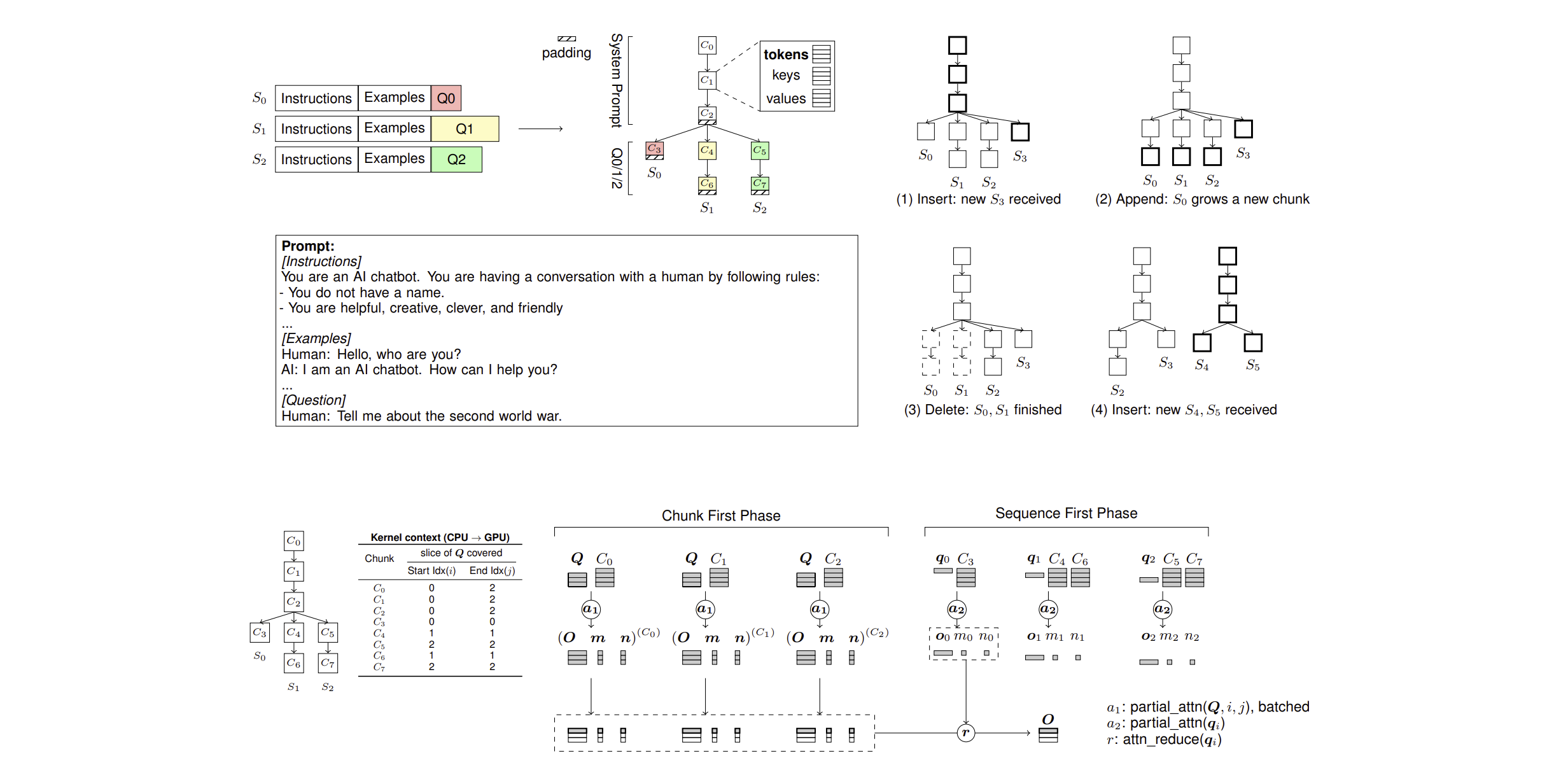
| ChunkAttention | PAKV exact-chunk lookup builds an active prefix tree; TPP separates shared and private chunks | shared chunks run chunk-first across covered queries; private chunks and reductions run sequence-first | identical leading token chunks among currently active sequences | concurrent active batches; 3.2–4.8× kernel throughput over PagedAttention, falling from 3.6× to 2.3× over that baseline at a 2K prefix as suffix length grows from 512 to 2,048 | completed-request state is outside the active tree, so tool gaps break continuity |
| FlashInfer cascade | prior grouping and page metadata yield block-sparse rows for shared and unique attention segments | cascade computes each segment in its efficient layout and combines exact attention states without moving KV | disjoint visible KV index sets; the caller supplies grouping/page metadata and FlashInfer derives sparse index/indptr views | composable over single-format kernel, suffix 128: 45.17 versus 46.52 μs gives about 1.03× at 1K/batch 16; 254.54 versus 4,090 μs gives 16.1× at 32K/batch 64 | the primitive does not discover graph or prefix groups |
| SGLang / RadixAttention | runtime longest-prefix match, persistent radix pages, leaf-LRU eviction, and cache-aware scheduling | avoids prefix recomputation across time and prioritizes longer current matches to increase cache-hit rate | exact token-sequence prefixes stored in paged KV; no concurrent batch is required for a later hit | reuse persists across arrivals; the one-month Chatbot Arena deployment observed 52.4% for LLaVA-Next-34B and 74.1% for Vicuna-33B, which are workload-specific token hit rates | it reacts after prefixes arrive and cannot make a shared decode prefix into one physical read across future branches |
Hydragen · declared exact-prefix batchingarXiv:2402.05099
Concurrent · declared treeInsight. When $b$ decode requests have one exact prefix, each has a different query but reads the same prefix K/V. Hydragen separates that prefix from each private suffix, stacks the queries, and turns the shared-prefix work from repeated matrix–vector operations into one matrix–matrix operation; per-segment LSE states then recover the exact undecomposed attention output (§3.1, Eqs. 2–5; §3.2, Fig. 1). The advantage is a scaling effect, not a constant multiplier. For CodeLlama-13B on 8×A100-40GB, Hydragen reaches up to 32× decode-only throughput over the best vLLM baseline at batch 1,024; at batch 32 with a 1K prefix and 128/256 generated tokens, it is only 1.06–1.11× over vLLM without detokenization (§4.1, Fig. 3; Appendix C.1, Tables 3–4). Prefill is excluded (Appendix D.1).
Where: $b$ is the number of concurrently decoded requests and $i\in\{1,\ldots,b\}$ indexes one request; $q_i\in\mathbb R^d$ is its one-token query and $Q\in\mathbb R^{b\times d}$ stacks all such queries; $d$ and $d_v$ are the attention-head key/query and value dimensions; $K_1,V_1$ are the one exact shared-prefix key/value matrices; $K_2^{(i)},V_2^{(i)}$ are request $i$’s private-suffix key/value matrices; $K^{(i)},V^{(i)}$ are their row-wise concatenations, denoted by $\Vert$; $j\in\{1,2\}$ selects a segment and $k_{j,r}$ is row $r$ of its key matrix (with $K_2=K_2^{(i)}$ for request $i$); $L_{i,j}$ is that segment’s scalar log-sum-exp normalization state; $\operatorname{SDP}$ is scaled dot-product attention; $O_i\in\mathbb R^{d_v}$ is the exact output. The diagram abbreviates the two segment outputs as $O_{i,1}=\operatorname{SDP}(q_i,K_1,V_1)$ and $O_{i,2}=\operatorname{SDP}(q_i,K_2^{(i)},V_2^{(i)})$; its $\oplus_{\mathrm{LSE}}$ denotes the displayed exact LSE-weighted merge. Exponentiation and scalar division broadcast across the $d_v$ value dimensions. The prefix term for all rows of $Q$ is executed as the shared matrix–matrix operation; the suffix term remains per request.
Hydragen · $b$ queries meet one physical shared-prefix KV block. The blue branch yields the K1 prefix state through an inter-sequence GEMM; purple branches retain request-specific suffix attention; green LSE fusion reproduces each full attention output. The figure claims amortized prefix traffic, not RelayAttention’s stricter one-read contract.
The next system uses the same exact segment algebra but a narrower service contract. Hydragen accepts an arbitrary caller-declared prefix hierarchy and improves arithmetic intensity; RelayAttention hard-codes one application system prompt and targets its repeated memory traffic.
Shortfall. The prototype requires the caller to declare the exact sharing tree, and useful inter-sequence batching still requires a sufficiently large compatible group before execution; it does not discover future workflow branches (§5).
RelayAttention · one fixed system-prompt relayarXiv:2402.14808
Concurrent · one applicationInsight. Ordinary batched attention rereads identical system-prompt K/V from off-chip DRAM/HBM for every request. RelayAttention places that fixed prompt in a separate cache, loads it once for a batched system-attention operation, computes a distinct system output for each distinct query, and combines it with that request’s private-context output using exact segment normalizers (§§3.2–3.3, Figs. 3–5; §3.3, Eq. 7; Appendix A, Eqs. 11–12). This is not reuse of one attention output. Against vLLM, vLLM-RA reaches up to 4.36× end-to-end throughput on noninteractive ShareGPTv3; interactive serving reaches about 2.2× sustainable request rate near 0.5 s/token with a 2K system prompt and up to 2.0× throughput on the Llama2-7B chatbot workload (§§4.2–4.3, Figs. 7–8).
Where: $b$ is the same-application batch size and $i\in\{1,\ldots,b\}$ indexes one request; $q^{(i)}\in\mathbb R^d$ is request $i$’s current decode query and $Q=[q^{(1)};\ldots;q^{(b)}]$ stacks them; $t$ is one representative request’s generation step, $s$ is the fixed system-prompt length, $u$ is that request’s user-prompt length, and $l=s+u+t$ is its visible sequence length; $j$ is a visible token position, and $1\le a\le e\le l$ are inclusive segment bounds; $q_t\in\mathbb R^d$ is the pre-scaled query, $k_j\in\mathbb R^d$ is a key, and $v_j\in\mathbb R^{d_v}$ is a value, with $d$ and $d_v$ the key/query and value dimensions; $K_{a:e},V_{a:e}$ collect positions $a$ through $e$; $\operatorname{Attention}$ is normalized dot-product attention on the stated segment, with query scaling absorbed into $q$ to follow the paper’s notation; $O^{\mathrm{sys}}_{1:b}$ denotes $b$ distinct system outputs produced by one batched operation; $\beta_t^{a\to e}$ is that segment’s scalar LSE; $\alpha_t^{\mathrm{sys}}$ and $\alpha_t^{\mathrm{ctx}}$ are complementary exact fusion weights; and $o_t\in\mathbb R^{d_v}$ is the full causal-attention output. In the diagram, $O^{\mathrm{ctx}}_{1:b}$ collects the distinct private-context outputs and $o_{1:b}$ collects their componentwise fusions with $O^{\mathrm{sys}}_{1:b}$. The first equation expresses batched execution, not output equality.
RelayAttention · The ordinary path issues one thin system-KV read per request. The relay path uses one thick batch read into the system GEMM, still emits distinct $O_i^{\rm sys}$ values, and fuses each componentwise with its corresponding $O_i^{\rm ctx}$ to produce $o_i$. GPU HBM is the off-chip DRAM shown here; it is not a second store.
Shortfall. There is no sharing benefit at batch one, gains diminish when private context is roughly twice the system prompt, and the implementation targets one common application prompt; multiple applications require IDs and same-application batching (Limitations; Appendix D).
ChunkAttention · active-batch prefix discoveryarXiv:2402.15220
Concurrent · discovered treeInsight. Exact sharing need not be declared before the kernel path. ChunkAttention’s Prefix-Aware KV Cache (PAKV) finds the longest exact leading-token path among sequences currently under decoding, while its Two-Phase Partition (TPP) traverses shared chunks chunk-first to preserve batched matrix operations and private chunks sequence-first to preserve locality (§§3.1–3.2, Figs. 1–2). The published method uses exact token-chunk lookup—not a specified PAT or hash interface. On A100-80GB with batch 32 and 64-token chunks, its decode kernel delivers 3.2–4.8× the throughput of PagedAttention for 1K–4K shared prefixes; at a 2K prefix, the ratio over that baseline falls from 3.6× to 2.3× as completion length grows from 512 to 2,048 (§4.1, Fig. 3).
Where: $S=(t_1,\ldots,t_{n_p})$ is one prompt’s token sequence of length $n_p$; $T$ is the CPU-side PAKV prefix tree over currently active sequences; $\operatorname{paths}(T)$ is the set of root-to-node paths, each formed by concatenating exact token chunks of capacity $c$; $P\preceq S$ means that path $P$ is an exact leading-token prefix of $S$; $|P|$ is its token count and $P^\star$ is the longest hit; $(K,V)_{P^\star}$ is the cached key/value state reused for that hit; $S[|P^\star|:]$ is the unmatched suffix whose K/V projections and position embeddings are computed and inserted. Prefill attention still reads the complete K/V sequence; the lookup skips only repeated state construction (§3.2).
Where: $C$ is one KV chunk of token capacity $c$; $S_i$ is active sequence $i$ and $\operatorname{path}(S_i)$ its PAKV path; $A_C$ is the contiguous set of active sequence indices covered by $C$ and $r_C$ its size; $Q\in\mathbb R^{b\times d}$ stacks one decode query per active sequence, $Q_{A_C,:}$ selects the covered rows, $b$ is active batch size, and $d$ is head dimension; $d_v$ is value dimension; $K^{(C)}\in\mathbb R^{c\times d}$ and $V^{(C)}\in\mathbb R^{c\times d_v}$ are chunk $C$’s keys and values; $W^{(C)}$ is its scaled score matrix; $\mathbf1$ is an all-ones vector; $E^{(C)}\in\mathbb R^{r_C\times c}$ is the row-shifted exponential-score matrix; $m^{(C)},n^{(C)}\in\mathbb R^{r_C}$ and $O^{(C)}\in\mathbb R^{r_C\times d_v}$ are row-wise maximum, exponential denominator, and unnormalized numerator. In the sequence-first recurrence, $o_i^{(C)},m_i^{(C)},n_i^{(C)}$ are sequence $i$’s slice of that shared state or a state computed for one private chunk; $O_i,m_i,n_i$ are its accumulated online-softmax state; $M,x,y$ are stable merge auxiliaries; and $\operatorname{Attn}_i$ is the normalized output. Algorithms 1–2 execute the first three lines by shared chunk, then the last two by sequence.
ChunkAttention · Exact-token chunks form a PAKV tree for active sequences. Each thick-blue spine chunk $C\in\{C_0,C_1,C_2\}$ is processed independently, chunk-first, against all covered queries and stores its own $(O,m,n)^{(C)}$ state; orange private branches run sequence-first and reduce with the corresponding state slices.
Shortfall. PAKV indexes only sequences under active decoding: when a sequence completes, its path is deleted and its chunks return to the allocator. A tool gap therefore breaks semantic continuity, and shared material must be a leading prefix (§§3.1, 3.3, 7).
FlashInfer · composable / cascade attentionarXiv:2501.01005
Composable · prior groupingInsight. Shared-prefix attention is one instance of a broader compositional rule: attention over any disjoint visible KV sets can be evaluated in different layouts and merged exactly. FlashInfer expresses heterogeneous shared and unique structure as block-sparse row (BSR) views, computes each level with a suitable query-row tile, and combines per-query attention states without moving KV; JIT compilation specializes the resulting kernels (§§2.2, 3.1.2, 3.2.3). The paper calls this attention composition and composable formats; cascade is the library API realization. In Appendix G.2’s suffix-128 kernel timings, single-format versus composable-format execution is 46.52 versus 45.17 μs at a 1K prefix/batch 16, so composable is about 1.03× faster; at 32K/batch 64 it is 4,090 versus 254.54 μs, or 16.1× faster. This is an intentionally extreme scaling contrast rather than an end-to-end expectation.
Where: $q,k_j\in\mathbb R^d$ are one query and visible keys, $v_j\in\mathbb R^{d_v}$ are values, and $d,d_v$ are key/query and value dimensions; $j$ indexes a visible KV entry and $i$ indexes a request; $\mathcal I,\mathcal J$ are disjoint visible KV index sets for the same query; $L_{\mathcal I}$ is the scalar per-query, per-head LSE; $O_{\mathcal I}\in\mathbb R^{d_v}$ is normalized attention over that set; $\mathcal S_{\mathcal I}$ is the two-part attention state, and $\mathcal S(q,K,V)$ denotes the same state evaluated for the stated query and KV matrices; $\oplus$ is its exact associative and commutative merge; $\mathcal S_i^{\mathrm{all}}$ is request $i$’s full state; $K_{\mathrm{shared}},V_{\mathrm{shared}}$ are shared-level KV and $K_i^{\mathrm{unique}},V_i^{\mathrm{unique}}$ its unique level. In the diagram, BSR row height $B_r$ is the number of query rows handled together and column width $B_c$ is the cache-manager page granularity. Given caller-supplied grouping and page metadata, FlashInfer computes index and index-pointer views that select existing pages, so composition does not relocate KV.
FlashInfer · A wide-row BSR view batches three queries over the shared level, while row-one BSR views cover unique levels; here $B_c=1$ page in both. Each produces a per-query state, and the green associative $\oplus$ composes the two-level cascade. The caller supplies grouping/page metadata, FlashInfer derives index and index-pointer views, and JIT specializes execution.
Shortfall. The primitive does not discover a workflow graph or decide which requests share a prefix; that grouping and prior knowledge remain runtime responsibilities, although FlashInfer can derive BSR index views from the supplied metadata. Its benefit can also be erased by merge overhead when the shared segment is short.
SGLang / RadixAttention · reuse across timearXiv:2312.07104
Persistent · runtime-discoveredInsight. Exact-prefix reuse is also a runtime retention and scheduling problem. Structured programs revisit identical leading-token histories after earlier calls finish, so RadixAttention retains prompt and generated KV in a CPU-indexed token radix tree, matches the longest prefix of each arriving request, evicts eligible leaves by LRU, and orders waiting work by longest matched prefix (§3, Fig. 3; Appendix A.2, Algorithm 1). This discovers reuse across time rather than requiring a concurrent batch. In a one-month Chatbot Arena deployment, token-level hit rates were 52.4% for LLaVA-Next-34B and 74.1% for Vicuna-33B; they reflect those two low-traffic, single-worker workloads, not a general production range (§6.2).
Where: $r$ is one request and $R$ is the offline request batch considered by the theorem; $x_r$ is request $r$’s exact input-token sequence and $n_r=|x_r|$ its prompt length; $t$ is a scheduling instant; $T_t$ is the currently cached radix tree; $\operatorname{match\_prefix}$ returns the deepest matched node $v_r$ and matched-token length $\ell_r$; $Q_t$ is the online waiting queue, and $\ell_r\downarrow$ means descending matched-prefix length with ties unspecified; $\pi$ is an execution order; $h_\pi(r)$ is the number of request $r$’s prompt tokens already cached when it executes; $H(\pi)$ is token-level cache-hit rate; $C_\pi$ is uncached KV computation in token units; $M$ is cache capacity in tokens; and $\pi_{\mathrm{LSPF}},\pi_{\mathrm{DFS}}$ are longest-shared-prefix-first and depth-first orders. The final line restates Theorem 3.1’s offline result under capacity at least the longest request; online arrivals disrupt DFS, so the paper presents the greedy order as an approximation and notes possible starvation (§3; Appendix A.3).
RadixAttention · Rebuilt from Fig. 3: an empty tree receives a chat, then requests hit, extend, and split exact-token edges. At step 7, the existing ‘What’ few-shot leaf remains grey while ‘When’ and ‘How’ are the two green insertions. Step 8 inserts $i$, evicts distinct nodes $g$ and $h$, and labels the retained few-shot leaves $j,k,l$. Step 9 hits $j$, retains one existing answer branch, inserts three green self-consistency answers, and evicts $i,k,l$. Blue marks a hit, green an insertion, grey retained state, and a dashed red cross an eviction; letters reproduce the paper’s node labels.
Runtime boundary. Prompt and generated KV share one page pool. A node’s reference count protects state used by running requests; only zero-reference leaves are eligible for LRU eviction, which preserves shared ancestors until they themselves become leaves. The paper’s overall 6.4× structured-program throughput headline also includes the language and runtime system, so it is not attributed here to RadixAttention alone.
Shortfall. Apart from a frontend $fork$ hint that can insert a declared prefix first, RadixAttention reacts only after exact leading-token histories arrive. It cannot foresee an unseen branch or turn a shared decode prefix into one physical read across active queries; its offline scheduling theorem also does not extend to online arrivals.
Layer conclusion. The decomposition point moves from a caller-declared hierarchy (Hydragen), to one hard-coded service boundary (RelayAttention), to an active-batch tree (ChunkAttention), to prior-knowledge composable segments (FlashInfer), and finally to a persistent runtime tree (RadixAttention). The saving correspondingly lands in arithmetic intensity, off-chip reads, traversal order, layout specialization, or cross-time recomputation. A dynamic MAS can combine persistent discovery with composable kernels and batch formation, but none of these systems predicts an unseen branch; every exact reuse still depends on identical tokens, positions, and visibility.
4. Serving layer: schedule programs, state, and uncertainty
The serving layer decides when requests run, where state resides, and which work is admitted or delayed. Building on the exactness constraints below it, this layer differs mainly in how much workflow structure it assumes and whether its policy is reactive, predictive, or admission-planned.
Five scheduling concepts recur here. A directed acyclic graph (DAG) is a dependency graph with no directed loop. Its critical path is the longest dependency chain that determines earliest completion. Prefetch moves state before its consumer arrives; a time to live (TTL) is a bounded interval after which retained state may be reclaimed. A structural signal is any application fact—identity, dependency, distance, or duration—that changes a serving decision.
The six designs form an information ladder, not a linear quality ranking. InferCept has no workflow graph beyond a pause plus runtime profiles. Autellix uses program identity and observed service history. Parrot exposes the currently submitted SemanticVariable dataflow and terminal criterion. KVFlow's frontend derives earliest step distances from a step graph. TokenCake combines a registered DAG with predicted tool duration, while Continuum learns a per-tool duration CDF from returns. A declaration, an observation, and a forecast carry different failure modes even when all are called agent-aware.



The table compares semantics and decision granularity: what the scheduler can infer, when it learns it, and what dynamic MAS behavior invalidates that inference. Section 5 separately inventories the concrete API fields, correctness rules, and portability of those interfaces.
4.1 Structure changes what the scheduler can decide
| System | Structural signal | Decision granularity | Information timing | What dynamic MAS breaks |
|---|---|---|---|---|
| Parrot | submitted SemanticVariable DAG + terminal performance criterion | request task group, placement, and prefix co-location | application-declared as functions unblock | client-side control can create unseen future nodes; cancellation or late growth changes groups |
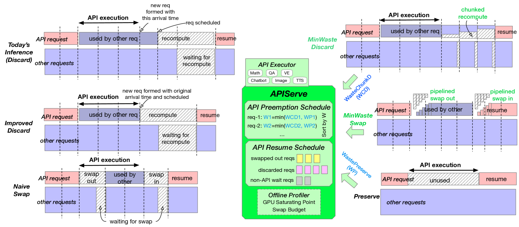
| InferCept | pause, context sizes, pause type/profile, elapsed estimate; no workflow graph | per-request KV action + global swap allocation | reactive at interception, using measured profiles | it cannot see the next consumer, branch probability, or critical path |
| Autellix / Agentix | program/thread ID + observed completed-call service; no future DAG | per-call queue/preemption by service score; routing by program identity and data locality | online attained-service history | new programs are cold; history cannot name the next call or prefetch target |
| KVFlow | current agent + frontend-derived earliest steps for every agent | radix-cache node eviction + candidate-agent prefetch | frontend-derived step vector sent with each request | runtime-created invocations absent from the vector make distances stale; OR branches may prefetch paths that never run |
| TokenCake | registered DAG/stage/importance + predicted and actual tool duration | per-block pool reservation + per-request migration timing | declared structure plus duration forecast and return event | late expansion is safe only when the frontend supplies updated metadata; timing error can make proactive transfers harmful |
| Continuum | program history + per-tool duration CDF + waiting queue | completed-turn KV retention TTL | history-derived forecast, overridden by an observed return | distribution drift, speculative branches, and context folding invalidate a tool-specific return-time bet |
4.2 Six serving mechanisms, paper by paper
ParrotarXiv:2405.19888
Declared dataflowInsight. Applications know their dataflow even when the serving engine sees isolated prompts. Parrot's SemanticVariable placeholders expose a bipartite request–value DAG, so the scheduler can reason backward from one terminal latency or throughput criterion, group parallel producers at a latency-sensitive fan-in, and co-locate requests with shared prefix structure (§§4.1–4.2, 5.2–5.4; Figs. 7–9). The abstraction exposes ends—values and performance goals—without forcing the application to prescribe an engine schedule.
Where: this is a per-terminal faithful formalization of Parrot §§4.1–4.2 and 5.2, not a numbered paper equation. $R$ is the submitted request-function set, $V$ the SemanticVariable set, $\sqcup$ a disjoint union, and $G_{\mathrm{SV}}$ their bipartite graph. $P_r$ is request $r$'s prompt template; $\operatorname{ph}_{\mathrm{in}}(v)$ and $\operatorname{ph}_{\mathrm{out}}(v)$ are the literal input/output placeholders for $v$, and $a\prec P_r$ means string $a$ occurs in $P_r$. $E_{\mathrm{in}}$ and $E_{\mathrm{out}}$ are the resulting edges. $v_o$ is one retrieved terminal output, $\kappa_o$ its latency or throughput criterion, $x$ a request or value ancestor, $\operatorname{Anc}_{G_{\mathrm{SV}}}(v_o)$ the ancestor set, $\operatorname{Anc}_R(v_o)=\operatorname{Anc}_{G_{\mathrm{SV}}}(v_o)\cap R$ its request ancestors, and $\kappa(x)$ the criterion propagated to $x$. $\operatorname{Pred}_R(r)$ is the immediate producer-request set feeding request $r$; $u\leadsto w$ means a directed path from producer $u$ to producer $w$. During latency traversal, a fan-in's multiple pairwise-incomparable—therefore parallel—producers form task group $\mathcal T(r)$. A throughput traversal marks direct and indirect producers throughput-preferred. The paper does not specify conflict resolution between different criteria attached to different terminals.
Boundary. The 11.7× headline is application-level latency against a latency-centric baseline (§8.4, Fig. 18), not a universal engine speedup: a simple chain is 1.38× versus vLLM (§8.2, Fig. 11), and mixed map–reduce is 1.05× versus the throughput-centric policy (§8.5, Fig. 19). Parrot's scheduler reasons over static or deterministically submitted DAG structure. Prompt content may be generated dynamically, but native/client-side control that creates unseen future nodes remains outside the cloud DAG (§6).
InferCeptarXiv:2402.01869
Pause + profileInsight. Interception is not termination: when a tool, retrieval, or human response returns, the request still needs its pre-interception context before appending the new result. Keeping, discarding, and swapping that KV each waste a different GPU-memory × time region, so InferCept models memory-time explicitly and chooses under a global swap budget (§§2.2, 3.2, 4.1–4.4). The scheduler needs no future request DAG, but it does use context sizes, an offline-profiled forward cost, a bandwidth-derived swap cost, pause-type hints, and an estimated or elapsed pause duration.
Where: $i$ identifies a request and $j$ its interception; $C_i^j$ is that request's context-token count at interception $j$, while $C_i$ is request $i$'s held context-token count in the preserve term, where the paper drops superscript $j$; $M$ is KV memory per token. $T_{\mathrm{fwd}}(x)$ is one forward-iteration time for $x$ tokens; $C_{\mathrm{other}}$ is the sum of all other running requests' context-token counts. $T_{\mathrm{INT}}^j$ is the pause duration, $T_{\mathrm{swap}}(x)$ the transfer time for $x$ tokens, and $C_{\mathrm{batch}}=C_i^j+C_{\mathrm{other}}$ the total batch context; factor two counts swap-out and swap-in. $n$ is the number of chunked-recompute iterations. Every $W$ is memory × time: $D$, $P$, $S$, and $\mathrm{ChunkD}$ denote raw discard, preserve, raw swap, and chunked discard. InferCept first assigns limited swap capacity globally in descending waste order; unswapped paused requests then use the printed preserve-versus-chunked-discard minimum $W_i^j$ (§4.3, Eq. 5).
Boundary. Across the mixed-workload model settings, InferCept sustains 1.6×, 1.8×, and 2× the vLLM arrival rate; the single-GPU 13B case reaches only up to 1.25× request rate without a noticeable normalized-latency increase (§5.1, Fig. 2). The reported 37–40% is recomputation's share of forwarding time under Discard, not a universal interception tax (§3.2 after Eq. 1). On the mixed workload, the elapsed-time estimator reaches 93% of an oracle supplied with exact interception durations (§4.4), but the policy still has no downstream consumer, branch, or critical-path signal.
Autellix / AgentixarXiv:2502.13965
Observed historyInsight. A request is the execution object, but the program is the accounting and fairness context: scheduling each call independently can delay one program's critical chain behind unrelated calls. Autellix, published as Agentix at NSDI 2026, therefore gives every arriving call its program's priority score. PLAS sums observed prior-call runtime; ATLAS refines this into a longest observed critical-path estimate without retaining dependency edges (§§4.1–4.2). Both are non-clairvoyant—future calls and runtimes are unnecessary.
Where: $c_j$ is the arriving $j$th model call; in PLAS, $c_k$ is a prior completed call in the same single-threaded program, while in ATLAS it is a completed parent of $c_j$. $\operatorname{id}(c)$ is the program identifier, and $t_k$ the measured executor runtime of $c_k$; $k$ precedes $j$ in PLAS call order. $p(c)$ is the scheduling-priority score numerically equal to attained service, with a larger value meaning lower priority. $\mathcal P(c_j)$ is the conceptual completed-parent set in the ATLAS recurrence; a root has none, but the implementation does not receive or retain these edges. $Q_i$ is attained-service queue $i$ among $K$ queues, bounded by $Q_i^{\mathrm{lo}}$ and $Q_i^{\mathrm{hi}}$; quantum exhaustion demotes a call. $W_p$ is accumulated program wait, $W_c$ current-call wait, $T_p$ program service, $T_c$ current-call model-execution time, and $\beta$ the anti-starvation threshold that promotes the program's call to $Q_1$. The paper does not specify numeric $K$, queue bounds, quanta, or $\beta$. Its printed PLAS subscript uses an undefined $c_i$; the first line follows the surrounding definition and corrects it to $c_j$.
Boundary. The reported 4–15× throughput range is against the default vLLM baseline, which lacks prefix caching in this setup, at equal program-level token latency. Against vLLM-opt, the homogeneous ShareGPT/BFCL and LATS workloads are 2×, while the final NSDI Mixed result is 5× (arXiv v1 reported 4×) (§6.3). A simplified simulator still shows a qualitative gap to clairvoyant SRPT (§6.5.3 / final Appendix A.2): history gives robust fairness but cannot reveal which call or branch comes next.
KVFlowarXiv:2507.07400
Step graphInsight. An agent workflow's near future can be represented as an Agent Step Graph: the frontend sends each agent's earliest steps-to-execution with the current agent, turning eviction from recency into graph distance (§3.1, Fig. 3). A fixed prefix needed in fewer steps receives stronger protection, while the backend prefetches possible next agents and overlaps transfer with current-agent GPU work (§3.2, Fig. 4). These distances are earliest-possible estimates, not clairvoyant knowledge of the realized branch.
Where: $v_{\land}$ and $v_{\lor}$ are synchronization and conditional nodes; $E_1,E_2$ are predecessor steps-to-execution and $s(v)$ is the earliest number of dependency-graph steps before $v$ can execute. The first line is KVFlow's §3.1 rule. The remaining lines faithfully formalize its prose eviction policy rather than quote numbered equations: $n$ is a radix-cache node, $\pi(n)$ its eviction priority, $a$ one agent invocation, and $\ell(a)$ that invocation's last fixed-prompt node; $m$ ranges over $n$'s child nodes. Shared prefixes inherit the minimum priority among descendant/end-point uses, including across workflows. $F$ is the set of fixed-prefix cache nodes, $\mathcal E$ the eviction sequence, $\Vert$ sequence concatenation, and $\operatorname{sort}^{\downarrow}$ descending order. Thus varying suffixes ($+\infty$) go first, then more distant fixed nodes.
Boundary. The 1.83× result versus HiCache uses a synthetic 10-agent sequential workflow with 8,192 fixed-prompt, 32 dynamic-input, and 32 output tokens per agent on one A10G (§4.1). In the realistic PEER simulation, the gain is up to 1.12× versus SGLang and up to 1.08× versus HiCache (§4.2). A runtime-created invocation absent from the supplied vector makes priorities stale; OR branches conservatively prefetch all candidates subject to an unspecified concurrency cap, and gains shrink when decode dominates.
TokenCakearXiv:2510.18586
DAG + durationInsight. Agent KV often idles while a function call occupies the application. TokenCake separates two questions that ordinary cache policies conflate: the spatial scheduler decides whose blocks occupy a shared or reserved GPU pool, while the temporal scheduler decides when a stalled request should offload and gradually preload (§§2.1, 4–5). Their cooperation protects graph-critical work without transferring KV when the predicted tool interval is too short to repay the round trip.
Where: $N_{\mathrm{blocks}}$ is the candidate request's KV-block count; $T_{\mathrm{offload}}$ and $T_{\mathrm{upload}}$ are measured device-to-host and host-to-device times, $T_{\mathrm{transfer}}$ their round trip, and $T_{\mathrm{FC}}$ predicted function-call duration. Passing this gate is necessary, not sufficient: a waiting request must use the freed blocks, CPU capacity must exist, and the policy score must permit offload (§4.2). $P_{\mathrm{upload}}$ is upload priority, $I$ normalized spatial importance, and $U$ return urgency. $B_{\mathrm{gpu}}^{\mathrm{free}}$ is total free GPU blocks, $D_{\mathrm{critical}}$ critical waiting demand, $B_{\mathrm{shared}}^{\mathrm{free}}$ free shared-pool blocks, and $B_{\mathrm{upload}}$ the safe upload budget. $B_{\mathrm{remain}}$ is that cycle's remaining budget, $B_{\mathrm{deficit}}$ the candidate's missing blocks, $\lceil\cdot\rceil$ ceiling, and $B_{\mathrm{reserve}}$ its new reservation (§4.3).
Boundary. The 47.06% mean end-to-end latency reduction is the Qwen2.5-14B CodeWriter D1 case versus vLLM at 1.0 QPS; at 0.05 QPS TokenCake is approximately at the baseline because memory contention is minimal (§7.2). With duration-noise scale $s=0.25$, it regresses by 8.3% relative to the agent/spatial-only variant (§7.5). The evaluated workflow graphs are static. A two-H20 tensor-parallel case appears in §7.1, but the paper leaves broader multi-GPU evaluation as future work (§9).
ContinuumarXiv:2511.02230
Tool CDFInsight. Multi-turn agents often return after a tool with a tool-specific empirical delay distribution. Continuum turns its CDF into a bounded retention bet by choosing the TTL that maximizes probability-weighted cache-hit benefit minus GPU-memory opportunity cost (§§3–4). The result is neither permanent pinning nor immediate LRU eligibility, but a per-request TTL with queue-aware release (§5.2).
Where: $f$ is the invoked tool type and $S[f]$ its observed duration sample multiset; the first $t$ is a sample, while the policy's $t$ is wall-clock time. $\mathbf1$ is an indicator, and $P(\tau,f)$ the empirical probability that tool $f$ returns within candidate TTL $\tau$. $r$ is a nonterminal LLM request whose output invokes a tool; $\operatorname{MemUsage}(r)$ is its GPU footprint and $\mathcal M$ the average active-request footprint, so $\operatorname{Cost}$ represents GPU-memory opportunity cost in aggregate-delay units and assumes a sufficiently full waiting queue. $\operatorname{CacheMissCost}$ covers reload or prefill after eviction; $\operatorname{OutofOrderCost}$ is the returning request's expected queue delay while it waits for GPU memory, which retention avoids; their sum is $\operatorname{Benefit}$. $\operatorname{uniq}$ returns distinct samples and $\tau^*$ the maximizing TTL. The final piecewise rule is a faithful normal-case formalization of §5.2, not a printed equation: $t_0$ is completion time, $\operatorname{id}$ the program identifier, $Q$ the waiting-request set, $q$ one waiting request, and $\pi_{\mathrm{TTL}}$ the retention action. A matching successor suppresses expiry until scheduling; termination unpins state, and allocation deadlock may evict pinned victims in latest-program-arrival order before their TTL.
Boundary. Continuum reports up to 8.18× lower delay in a real SWE-agent testbed experiment, but the cross-setup range is 1.12–3.66× across three hardware/model configurations (§6). Its cost model assumes each tool's historical latency distribution remains useful; drift or adversarial volatility can spoil the TTL, while speculative branches and context folding require policy changes (§7; Appendix D).
4.3 Recent systems make structure and feedback partial
Newer systems occupy intermediate points rather than a graph-known/graph-unknown binary. Orla adds a stage DAG and coarse state hints; Helium compiles structured programs into joint operator/cache/schedule plans; Policy Runtime (CacheSage) learns next-agent transitions; Dyserve commits only the admitted portion of a finite plan; AAFLOW+ makes state lineage explicit; and InfraMind closes the loop from live load to topology, although its implementation is proprietary. The table records the scheduling consequence and evidence boundary. Section 5 owns the exact interface inventory, so those wire-level fields are not repeated here.
| System | What it adds | Evidence boundary | Remaining limitation |
|---|---|---|---|
| Orla | stage/dependency DAG and coarse preserve-or-flush hints across SGLang, vLLM, Ollama, and a simulator | preprint; lower boundary is multi-backend but Orla-specific | no exact token lineage, cancellation contract, or portable feedback semantics |
| Helium | compiled workflow DSL, mixed-integer linear programming (MILP) over discrete and continuous planning choices, proactive KV, and cache-aware scheduling on vLLM 0.16.0 | up to 1.56× versus KVFlow, while the proactive-KV ablation alone changes 130.14 s to 134.76 s, a 3.55% contribution | compiled AgentScope programs and one modified engine; dynamic expansion is not the evaluated mode |
| Policy Runtime / CacheSage | online first-order next-agent probabilities for eviction and prefetch | 13–37 percentage-point hit gain, 6–26% lower per-turn E2E latency, and 6–14% throughput gain; an abstract-level 12–29% TTFT claim is not supported by a defined or plotted TTFT metric | fixed role inventory, short historical horizon, and no exported exact future graph |
| Dyserve | admission compilation over model, verification, and live-load choices, with later pressure-aware rung shifts | on four tasks, accuracy rises 3–10 points over the strongest-accuracy baseline at 1.1–6.8× lower latency; one burst setting’s goodput changes from 25.7% to 67.2%, while a different fleet sees no shifts | branches must be resolved and loops bounded at admission; later expansion requires another compilation |
| AAFLOW+ | separate data and state edges with materialize, transfer, fork, restricted compose, and evict operations | reported TTFT tables combine analytical traces and measured microbenchmarks; they are not production end-to-end runs | AAFLOW-specific, not a portable standard; composition is limited to compatible non-overlapping sequential spans |
Across the six mechanisms, more structure buys earlier and finer action but creates a sharper stale-information failure. Pause-local InferCept can only react, yet an unexpected branch does not invalidate a graph it never stored. Autellix's history survives arbitrary control flow but cannot prefetch a named successor. Parrot can group the submitted dataflow; KVFlow can rank cache nodes by earliest use; TokenCake can time block movement; Continuum can bound a finished turn's residence. Each added step depends on a stronger claim about what comes next.
Decision granularity is equally important. Autellix shares accounting at program scope while still executing calls; InferCept acts on one paused request under a global swap budget; Parrot groups requests; KVFlow ranks radix-tree nodes and candidate agents; TokenCake reserves blocks across two pools; Continuum governs completed-turn state. Dynamic MAS can change topology, cancel work, fan out, merge asynchronously, or shift tool latency faster than any one of those units updates. No cache-node policy repairs a stale program graph, and no program priority identifies which KV block will be consumed next.
Layer conclusion. Serving systems differ less by an agent-aware label than by the validity window and decision granularity of their information. Submitted dataflow supports grouping, attained history supports non-clairvoyant fairness, step and duration forecasts support proactive state movement, and tool CDFs bound retention. Dynamic workflows need those claims to be refreshed or revoked; Section 5 asks whether today's interfaces can express that contract without tying the application to one runtime.
5. Interfaces that already exist
The layer comparisons reveal that information already crosses several application–engine boundaries. This section therefore replaces a binary absence claim with a precise interface ledger: accepted structure, correctness semantics, engine portability, and the remaining contract.
The earlier claim that no interface exists was too broad: several partial interfaces now exist, but none supplies the portable bidirectional contract described here.
Four interface terms recur in this section. An application binary interface, or ABI, is a stable machine-to-machine contract; here it is used broadly for the boundary between orchestrator and engine. A request for comments, or RFC, is an open design proposal rather than a merged feature. Correctness semantics determines whether a state operation is exact, approximate, rejected, or recomputed. Portability asks whether the same metadata can cross frameworks and engines without adopting one system’s compiler or modified endpoint.
| Interface | What it accepts | Correctness semantics | Portability | What it still omits |
|---|---|---|---|---|
| Parrot Semantic Variables | declared value dependencies, request functions, and application objectives | semantic values are explicit, but KV lineage and compatibility are not an external ABI | Parrot programming model and service | incremental graph growth, cancellation, and infrastructure feedback into topology |
| TokenCake DAG frontend | registered Graph DAG with LLMNode and FuncNode, edges, function Stage lists, and predicted duration; call_start sends request ID and initial estimate, while call_finish returns actual duration | critical-path and duration semantics guide reservation and movement; no exact token-state lineage | modified vLLM and OpenAI endpoint; TokenCake-specific | partial updates, dead-branch cancellation, exact lineage, and cache-pressure feedback to graph choice |
| KVFlow Agent Step Graph | invocation nodes, dependency edges, AND aggregation by maximum distance, OR aggregation by minimum distance, current agent, steps-to-execution for every agent, unique client ID, and fixed-or-dynamic-prefix information | graph-step distance is well defined; token identity, state compatibility, and cancellation are not | SGLang 0.4.4 and sgl.function-specific | incremental topology, lineage, cancellation, and engine-to-orchestrator feedback |
| Pythia workflow metadata | workflow_type_id, workflow_id, and agent_id in extra_body.app_metadata; the profiler adds a predicted output-length interval, predicted path regular expression, and prompt-composition pointers containing request ID, request-or-response selector, and token range | metadata identifies lineage sources for prediction; rare transitions below 5% are pruned and reactive fallback handles unsupported paths | framework-agnostic interceptor, but modified-SGLang and backend-specific implementation | exact graph facts, cancellation, state fingerprint, and feedback that can alter topology |
| SGLang agent-aware KV RFC #24656 | an outer agent_hints object with exactly twelve fields: workflow_id, agent_id, step_id, step_index, total_steps, parent_step_id, children_step_ids, tool_name, expected_tool_duration_ms, cache_ttl_ms, shared_prefix_hash, and reuse_hint | hints do not establish exact lineage or compatibility; hash reuse and storage inheritance are explicitly outside the proposal | open, unmerged RFC; pull requests (PRs) #24993 and #29199 remain open and the schema is being redesigned toward trajectory or session semantics | cross-process coordination, production scoring, exact lineage, cancellation, and bidirectional policy |
| Orla lower boundary | full stage/dependency DAG, schedule hints, and coarse preserve-or-flush state control | stage dependencies are explicit; exact KV identity and composition are not | OpenAI-compatible boundary over SGLang, vLLM, Ollama, and a simulator, but Orla-specific | exact lineage, cancellation, and standardized feedback |
| Dyserve compiler boundary | materialized finite DAG, node metadata, backend catalog, and live load at admission | unresolved branches are rejected, loops are bounded or unrolled, and later expansion is a new compilation; committed prefix is preserved while the uncommitted physical suffix may change | Flow and LangGraph adapters over a proprietary compiler | progressively revealed and open-ended graph growth within one compilation |
| AAFLOW+ state graph | separate data and state edges; state records model and configuration, layer, block, token position, positional metadata, lineage, placement, and ownership | materialize, transfer, fork, restricted compose, and evict; unknown compatibility causes replay or recomputation; merge is limited to non-overlapping sequential concatenation under lineage and compatibility | AAFLOW-specific state runtime; not a cross-engine standard | portable event versioning, application cancellation, policy feedback, tenant boundaries, and production validation |
Taken together, the missing object is narrower and more demanding than a graph API. It is a cross-framework, cross-engine, incrementally updatable, bidirectional ABI with explicit correctness semantics; partial graph updates and cancellation; exact token and state lineage; tenant, security, and failure rules; and measured infrastructure feedback that an application-authorized policy may use. No audited interface supplies that complete set.
The four figures below show how Dyserve, Orla, Helium, and the Policy-Driven Runtime Layer place that partial boundary in concrete stacks.


6. Master census: a dated research map
The layer analysis now returns to the full corpus so that highlighted systems do not displace adjacent work. This table preserves every work in a census this project compiled and then audited with two independent reviewers (process in §14), and adds the papers verified during that audit.
The structure column records what becomes available to infrastructure, not whether a paper uses the word dynamic. Evidence cells state mechanism or scope and avoid treating incomparable headline ratios as a ranking. Preprint labels are retained where archival venue claims were not verified.
Scroll horizontally for all six columns.
| Work · identifier | Status | Primary layer | MAS scope | Structure available | Focus or evidence boundary |
|---|
Part II · Why dynamic MAS matters
Structure is useful only when its availability time is stated
Part I showed that existing systems consume different forms of structure. Part II classifies when that structure exists, derives the facts–hints–feedback conclusion from measured evidence, and then marks the correctness boundary that information alone cannot remove.
7. What dynamic means: four workflow-knowledge types
A single dynamic label hides four different information schedules. This taxonomy is placed here because the interface ledger establishes that optimization depends not only on which graph exists, but on whether it exists at admission, during execution, or only after external observations.
Three objects must remain separate. A potential graph is the search space of allowed roles and edges. A realized control graph is the concrete set chosen for one workflow. An exact future trace additionally contains timings, token identities, tool returns, retries, cancellations, and page accesses. Knowing the first does not imply knowing the second, and knowing the second does not imply the third.
The new diagram depicts the four availability patterns. Solid edges are committed for the current instance; dashed edges are known possibilities whose outcomes remain unresolved; red observations introduce choices that did not exist at admission. A compiled program can therefore be fully available while its data-dependent realized path is not.
The adjudication table grounds each type in method text and links every primary paper. Monte Carlo Tree Search, or MCTS, is a search procedure that scores workflow candidates through repeated tree expansion and evaluation. A supernet is a graph that contains the candidate operators and edges from which one concrete subsystem can be sampled. The corrected DyLAN identifier is 2310.02170, published at COLM 2024; the earlier 2302-series identifier was wrong.
| Paper or mode | Type | Verified evidence snippet | Infrastructure consequence |
|---|---|---|---|
| AFlow · 2410.10762, evaluated mode | A · compiled | “each tree node represents a complete workflow” | MCTS returns a fixed workflow before evaluation; its code may still contain conditionals. |
| GPTSwarm · 2402.16823 | configuration-dependent | samples “whether to include edge ei in G′ for all i’s” | The learned edge distribution is query-independent; the realized DAG is complete before topological execution. Thresholded reuse is compiled, while per-run resampling resembles query sampling. |
| MaAS · 2502.04180 | B · query-sampled | “a task-specific multi-agent system G is generated and executed” | Sampling depends on the query and previously sampled operators, not execution outputs; the realized graph exists before dispatch. |
| G-Designer · 2410.11782 | B · query-sampled | the Design stage “decode[s] the communication graph topology” | The Optimize-stage collaboration receives a complete query-specific graph. |
| MasRouter · 2502.11133 | B · query-sampled | “samples the customized components … After executing the sampled MAS” | Mode, roles, and models are chosen before execution; later feedback trains the router rather than creating the current graph. |
| DyLAN · 2310.02170, COLM 2024 | C · progressively revealed | “edges will only be added for these top-ranked agents” in the next step | Runtime responses and ranking determine the next frontier; a complete realized graph does not exist at admission. |
| ReAct · 2210.03629 | D · open-ended | reasoning and task-specific actions occur “in an interleaved manner” | At each step an external observation precedes the next action; later actions and edges do not yet exist. |
| AutoGen · 2308.08155 | spans A, C, and D | GroupChat performs “dynamically selecting a speaker, collecting responses … and broadcasting the message” | Static flows are compiled; dynamic speaker selection is progressive or open-ended. The mode, not the framework name, determines the type. |
The type determines which optimizations are even possible. Type A permits program-level planning, meaning that the scheduler can coordinate several calls as one declared program, but distance-aware eviction, the KVFlow mechanism above, and exact branch grouping, which groups branches only when their token sequences and recorded histories match, apply only to committed edges with exact lineage; a compiled conditional may still be unresolved. Type B permits those actions over the admission-realized control graph, again only where lineage is exact, while future timings and tokens remain unknown. Type C permits frontier updates and factual cancellation, meaning removal of a branch after an observed event proves it will not run, while hints remain necessary for unresolved edges. Type D permits only current lifecycle facts, tool-conditioned TTLs, calibrated prediction, in which predicted probabilities match observed frequencies, and reactive fallback.
The available deployment evidence is uneven across these four types. Open-ended traces are much more visible than progressive traces, compiled programs appear mainly in controlled systems, and deployed query-sampled traces are nearly absent; no defensible deployment percentages exist.
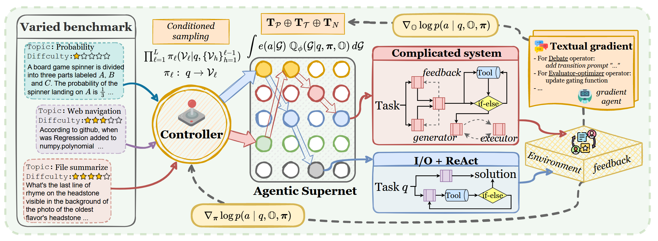
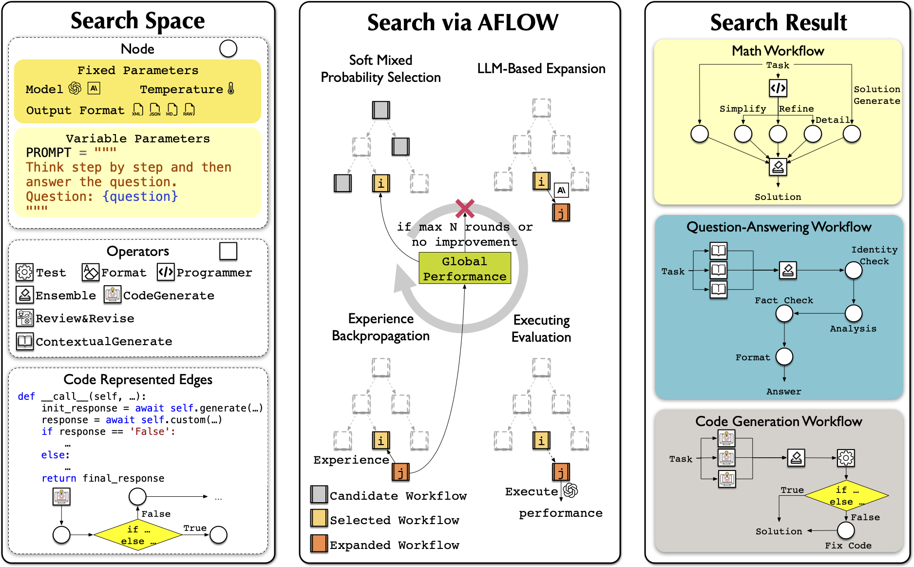
8. The information gap, restated: facts + hints + feedback
The four types rule out a universal choice between graph export and prediction. This section derives a closed-loop thesis from three measured cases: static graph facts help KVFlow, prediction recovers value beyond those facts in PBKV, and Pythia coordinates longer-horizon hints while admitting a reactive limit.
The measured thesis is that facts help most when the workload exposes them and pressure makes retention choices consequential, while prediction adds value for the unresolved remainder. KVFlow demonstrates the value of a known graph, but its 1.83× and 2.19× stress results become 1.08–1.12× on realistic PEER. PBKV uses GraphSAGE, a graph neural network that aggregates neighboring-node features, to make query-conditioned forecasts. It reports up to 1.85× E2E over least-recently-used eviction, or LRU, which discards the cache entry unused for the longest time, on dynamic workflows. On a static FinanceBench workflow, a financial document-analysis benchmark, PBKV reports 1.26× E2E with 1.39× hit rate over KVFlow; below 60 concurrent workflows, all compared policies are similar. Predictor accuracy declines from 0.935 at one step to 0.771 at three steps, so the value is workload-, pressure-, and horizon-dependent.
Pythia uses three identity facts to mine output-length intervals, prompt lineage, and recurring path grammars. It reports up to 2.9× lower JCT and 1.96× throughput, while the low ends are 1.38× JCT, 1.15× P95, and 1.12× throughput; curves converge at low load. It also states that unconstrained meshes force reactive behavior. Prediction is therefore a complement for residual uncertainty, not a substitute for facts that already exist.


Rebuilt historical diagram. The following SVG retains the original page artifact in a vertically stacked, legible layout. Its rightmost “missing” label and its caption’s claim that no interface exports a live graph are superseded by §5: partial interfaces exist, and the remaining gap is a portable bidirectional correctness contract.
The corrected synthesis needs a loop rather than a ladder. Facts move downward as committed structure and exact lineage; hints cover unresolved futures with probability and expiry; feedback moves upward as measured queue, cache, transfer, and compute state. The application retains authority over whether infrastructure state may alter topology or only influence physical execution.
Evidence-derived thesis. Export knowable facts as soon as they exist; predict only the residual uncertainty; return measured infrastructure state under an application-authorized policy; degrade to reactive when neither facts nor calibrated prediction are available.
Feedback is the least established leg. TokenCake returns actual function duration to its estimator. Dyserve replans only an uncommitted physical suffix from queue telemetry. InfraMind is the nearest topology-feedback implementation, but the implementation is proprietary. The experiment in Part III tests the marginal value of facts and hints for eviction; it does not validate this feedback leg or the full control plane.
9. Fan-in, when several parents converge: four correctness cases
More graph information can improve placement and retention, but it does not make arbitrary KV composition correct. This section follows the closed-loop thesis with the safety boundary: fan-in, meaning several parent branches converging on one consumer, has four distinct semantics.
The three-column diagram groups exact textual serialization and exact readout in one safe-side panel, with readout shown as an inset. The prose and table retain four cases because readout composition is exact for an attention query over separate parent segments but does not recreate a continuation in which parent tokens conditioned on one another. A canary is a deliberately sensitive test route used to detect quality regression before wider use.
| Case | What is exact | Required condition | Safe policy |
|---|---|---|---|
| 1 · Exact textual serialization | the consumer sees canonical parent text in one ordinary prompt | deterministic order and serialization; only the exact common ancestor is a cache hit | prefill every changed suffix; treat summarization as a separate lossy application operation |
| 2 · Exact READOUT merge | one query’s attention readout over separate parent segments can be merged with LSE state | the intended mask lets the query read those unchanged segments independently | use as a read operation; do not claim it recreates cross-parent conditioning |
| 3 · Structurally exact continuation | reused tokens have identical tokens, positions, causal predecessors, masks, model configuration, and lineage | normally a single parent or non-overlapping sequential concatenation already present in lineage | reject unknown compatibility and replay or recompute |
| 4 · Approximate repair | nothing is exact beyond declared unchanged spans; repair estimates missing conditioning | route-matched qualification, reasoning-heavy canaries, drift monitoring, and an exact fallback | keep outside the correctness ABI until separately validated |
The measured losses justify the conservative boundary. KVLink reports up to 35% relative QA loss for naive concatenation. On Natural Questions, an open-domain QA benchmark, positional re-encoding alone yields 28.9 F1 versus 72.5 F1 for the full reference, showing that RoPE correction is insufficient. Kamera reports retrieval accuracy falling from 0.74 to 0.38 and multi-hop accuracy from 0.41 to 0.28 in binding-heavy settings, while its dense-text MuSiQue case, a multi-hop QA benchmark, shows no gap. KVCOMM loses up to 9.2 percentage points on AIME, a competition mathematics benchmark, even though MMLU, a multi-subject knowledge benchmark, can remain unchanged. Route-matched tests are therefore necessary because an easy aggregate benchmark can conceal the failure mode.
Part III · Design and experiment
A research-scale boundary with a falsifiable first test
Part II established the information schedule and correctness boundary. Part III narrows the proposal to one lab’s implementation, states hypotheses before results exist, and separates the eviction experiment from the untested feedback architecture.
10. A minimal control-plane design for research scale
The feasible design is not a new distributed platform. It is a small versioned control boundary in one engine that separates graph facts, graph hints, and runtime feedback, and applies exact reuse before any approximate transformation.
The control boundary is an ordered, idempotent event log: replaying an event produces the same state, and a cancellation supersedes prior intent without silently rewriting history. Hints never assert correctness. Feedback never changes application semantics unless an explicit policy grants that authority.
The table below lists the three control channels, one row per channel, with their minimum fields and contracts.
| Channel | Minimum fields | Contract |
|---|---|---|
| FACT | event version; workflow, node, and edge IDs; commit, completion, cancellation, termination; exact token-prefix lineage and consumers | immutable observation; may establish exact next-use rank only where the graph proves it |
| HINT | possible node or edge; probability; horizon or TTL; provenance; calibration version | expires automatically; cannot establish lineage or permit approximate reuse |
| FEEDBACK | queue delay; cache residency and pressure; tier and transfer cost; compute availability; measured duration | advisory unless an application-authorized policy maps it to topology choices |
10.1 Compatibility fingerprint and exact-first staging
A state fingerprint is the set of fields that must match before reuse can be called exact. No audited system checks the whole set, so the proposed prototype logs it even when the first experiment uses ordinary vLLM hash matching.
- Checkpoint and configuration, tokenizer and exact token IDs, KV dtype and layout, layer, block, and token position.
- RoPE configuration, causal predecessors, attention mask and visibility, modality, and complete state lineage.
- Tenant and authorization domain, retention policy, and semantic-deletion scope so that a valid numerical hash cannot cross a forbidden boundary.
Execution is staged conservatively. First, reuse only an exact prefix. At fan-in, canonically serialize parent text, reuse only the exact common ancestor, and prefill the remainder. Keep approximate repair outside the correctness ABI and require route-matched qualification plus exact replay fallback. When neither facts nor calibrated hints exist, use ordinary recency-based execution.
10.2 One-lab implementation boundary
The proposed build contains one common eviction scorer, four information adapters, versioned logging, and an inactive-prefix arena in one vLLM engine. It does not implement cross-engine transport, topology mutation from feedback, distributed recovery, or approximate state composition. Raw token IDs and prefix hashes are treated as sensitive metadata.
Architecture status. This control plane is a research synthesis, not an end-to-end validated architecture. Its proposed cache value $V(s)$, a scalar score for retaining state $s$, is unvalidated and mixes quantities unless every term is normalized to a common cost unit. PBKV’s survival score and Continuum’s Benefit-minus-Cost TTL are narrower precedents. Production work would still need capability negotiation, feedback stability, authorization, encryption, semantic deletion, backpressure, crash recovery, and rollback.

11. Observed problems and pre-registered hypotheses
The first experiment should answer one disputed systems question rather than attempt the whole architecture. Holding cache actions fixed, it measures the marginal value of recency, historical hints, currently knowable graph facts, and oracle future information.
No audited paper isolates those four information levels under the same token stream, cache capacity, page granularity, request schedule, and eviction action. The observed problem is therefore a missing controlled contrast, not an assumption that graph facts must outperform prediction.
Four workloads and four information levels define the comparison. The compiled workload (W1) fixes the program before admission; the query-sampled workload (W2) selects one complete graph before execution; the progressively revealed workload (W3) commits only the next frontier as responses arrive; and the open-ended workload (W4) can introduce choices after external observations. Reactive recency (L0) uses only current cache state and recency; history hints (L1) add learned transition probabilities; exported facts (L2) add currently known nodes, edges, lineage, consumers, completions, and cancellations; and the future-trace oracle (L3) adds the exact future page-access trace.
H1 · History under progressive revelation
Under the progressively revealed workload (W3), history hints (L1) versus reactive recency with no future information (L0) must improve steady-state GPU token hit rate by at least 5 percentage points.
H2 · Facts add value beyond prediction
Across the compiled workload (W1) and query-sampled workload (W2), weighted equally, exported facts (L2) versus history hints (L1) must reduce miss-prefill tokens per workflow by at least 5%, with neither workload worsening. Miss-prefill tokens are prompt tokens that had to be recomputed because their cache entry was not resident.
H3 · Facts have user-visible value
Across the compiled workload (W1) and query-sampled workload (W2), weighted equally, exported facts (L2) versus reactive recency (L0) must reduce mean per-agent TTFT by at least 5%, with neither workload worsening.
H4 · Residual gap in open-ended work
Under the open-ended workload (W4), the future-trace oracle (L3) versus exported facts (L2) must improve steady-state GPU token hit rate by at least 5 percentage points. The future-trace oracle (L3) is a ceiling, not a deployable baseline.
The 5% or five-point margin is a pre-registered smallest meaningful effect, not a parameter copied from one paper. It is below CacheSage’s weakest reported 13-point hit and 6% latency changes, near Helium’s isolated 3.55% proactive-KV contribution, and below KVFlow’s realistic 1.12× upper comparison.
The compiled workload (W1) having exported facts (L2) close to the future-trace oracle (L3) is a diagnostic expectation only. An equivalence margin is a pre-set tolerance used to conclude that two effects are practically the same; none is defined here, so this expectation is not a fifth hypothesis.
12. Experiment design, provenance, and decision rules
The experiment tests the four hypotheses in §11 through an eviction-only value-of-information study on one RTX 5090. It disables CPU offload, request reordering, topology changes, approximate KV transforms, and speculative prefetch so that information level is the only changed input to one common eviction path.
All levels reuse only exact vLLM hash-matched prefixes. Fan-in is canonically serialized as text; parent tensors are never merged. Greedy output token IDs must match across levels, so a content difference invalidates the run rather than becoming a latency observation.
12.1 Four workloads and four information levels
Each workload instantiates one type from §7 with an exact reveal rule. The harness may hold a prerecorded future for pairing, but L0 through L2 receive only what an online execution would know at that moment.
A tape is a frozen, replayable recording of arrival times, request order, and tool gaps; using the same tape makes level comparisons paired.
| Workload | Realization | Reveal rule |
|---|---|---|
| W1 · compiled | fixed 12-agent chain; 20 workflows per cell | L2 receives every node, ordered edge, exact role-prefix lineage, and consumer at admission. |
| W2 · query-sampled | complete ordered DAGs with 2, 3, 4, or 5 agents; five workflows of each size | The whole realized DAG and exact prefix consumers arrive before the first node dispatch. |
| W3 · progressive | six-agent AutoGen SelectorGroupChat; 50 warm-up paths and 20 measured paths per tape | Only the current node and newly committed next-speaker edge are released before dispatch. |
| W4 · open-ended | 20 mini-swe-agent sessions per tape from a frozen 100-session public corpus, split 50/50 for warm-up and measurement | Current session, exact lineage, tool call, observed return, and cancellation appear only when they occur; L3 alone receives the future page trace. |
The information ladder holds page size, recency clock, score/update path, first-come-first-served request order, cache capacity, and tie-breaking constant.
Three cache rules define the comparison. Automatic prefix caching, or APC, identifies exact reusable prompt blocks; least recently used, or LRU, evicts the block untouched for the longest time. A recording pass supplies Belady’s farthest-next-use order for L3; Belady is an offline rule that discards the item whose next use is farthest in the future.
The common eviction contract makes that control explicit. At every level, $S(b)=r_{\mathrm{norm}}(b)+w_{\mathrm{pred}}u_{\mathrm{future}}(b)$ with $w_{\mathrm{pred}}=1.0$, following CacheSage’s scorer structure. Only rank order is shared, so the numerical calibration need not match across levels. The engine evicts the lowest-ranked unreferenced block; recency breaks ties; active or referenced blocks are never evicted. L1 predictor state is $(workflow\_type,agent\_id)$ and appends the emitted tool name on W4; its hint expires at the next observed transition.
The table below lists the four information levels, one row per level, from reactive recency through the future-trace oracle.
| Level | Information | Common scorer input |
|---|---|---|
| L0 · reactive | exact token hash, residency, reference count, recency | future utility is zero; policy reduces to block LRU/APC |
| L1 · hints | L0 plus CacheSage-style first-order state-transition probability | probability expires at the next observed transition and never asserts lineage |
| L2 · cumulative facts + hints | L1 plus currently known nodes, edges, exact lineage and consumers, completion, and cancellation | proven graph-step rank overrides hints only where facts establish it |
| L3 · oracle | L2 plus exact future page access or non-access | Belady rank through the same eviction call; it is not deployable |
The main grid contains $4\times4\times10=160$ cells: four workloads, four levels, and ten paired arrival/order tapes. Each cell has 20 workflows. The tape, not an individual cache-correlated workflow, is the inference unit. The primary mechanism metrics are steady-state GPU token hit rate and miss-prefill tokens per workflow; mean per-agent TTFT is the user-visible metric. Serving-only JCT excludes recorded tool sleep, while E2E JCT including tools is secondary.
W4’s frozen measurement pool contains 50 sessions, so sessions necessarily recur across ten 20-workflow tapes. Tape-level resampling preserves within-tape cache dependence; it does not make the underlying sessions independent. The W4 inference therefore applies to this frozen reproduction corpus, with session IDs and observed statistics published for audit.
The paired execution contract freezes identical pretokenized requests, W2 graph samples, arrival and order tapes, reveal events, and recorded W4 tool gaps across L0–L3. Cache state is flushed between cells while model weights remain loaded. A balanced randomized level order within each tape limits thermal and time drift, and no comparison mixes engine builds.
The implementation fixes one exact copy of the serving engine and records its version so results can be reproduced; a brief pre-run check confirms that the code runs on the target GPU generation; only Python-level policy code is changed. Only after a clean main grid do labeled, non-pooled secondary cells test a 4,096-token prefix, a 1,024-token output, a PBKV-style Markov lookahead for L1 that looks ahead three steps and discounts each further step’s influence by 0.7, and equal-budget conservative prefetch using only free space and cache space retired from active use at every level.
12.2 Parameter provenance and design-choice registry
Every harvested workload or system value below names a source paper and location. The same registry also includes every statistical, integrity, build, and scope choice for which no source paper supplies the chosen value; those rows say so explicitly because attributing them to a paper would fabricate provenance.
| Parameter | Our value | Source paper | Where stated |
|---|
Composite arena derivation. Let $B_{\mathrm{profile}}$ be profiled inactive blocks. The reclaimable arena is $$\min(\lfloor .5B_{\mathrm{profile}}\rfloor,\;8192/16)=\min(\lfloor .5B_{\mathrm{profile}}\rfloor,\;512)$$ blocks. TokenCake supplies the 0.5 pressure anchor and 16-token block; Helium supplies the 8,192-token limit. No cited paper used this exact inactive-only composite.
Rows marked “No source paper” are pre-registered design choices, not missing citations. Keeping them in the registry makes the complete protocol auditable while preserving the distinction between a borrowed experimental anchor and a new decision.
12.3 Pressure preflight and PASS criteria
A cache experiment is uninformative when everything fits or when active requests are forced out. The preflight therefore selects pressure before comparing levels. A Poisson arrival process models independent arrivals at a fixed mean rate; the five candidate rates below are TokenCake’s published grid.
- For each workload, run one fixed L0 tape at TokenCake’s five published Poisson rates: 0.05, 0.1, 0.2, 0.5, and 1.0 workflows per second.
- Freeze the lowest rate whose interior interval — the stable measurement window after warm-up and before drain, where evictions and later reuse can both still occur — contains an inactive-block eviction and at least one candidate with proven later exact reuse.
- Require zero out-of-memory events and zero active-page preemptions. All ten main L0 tapes must retain a valid interior interval.
- If no published rate passes, report “pressure design invalid” and do not introduce a new rate after observing effects.
For each hypothesis, compute one paired difference—the difference between two levels on the same tape—per tape. The run-cluster paired bootstrap re-draws the ten tapes with replacement 10,000 times to measure how much the average difference varies while preserving within-tape cache dependence. Holm correction then adjusts the four hypothesis comparisons to keep the probability of any false positive across the four tests at $\alpha=.05$. PASS requires the adjusted lower 95% confidence bound—the pessimistic end of the uncertainty range after correcting for testing four hypotheses—to clear the full five-point or 5% margin; excluding zero without clearing that margin is FAIL. H2 and H3 additionally require neither workload’s point estimate, the single best estimate from the observed data, to worsen.
Reporting includes every per-tape effect, mean, median, standard deviation, and adjusted interval. A p-value is the probability, under the null model, of a result at least as extreme as the observation; it is never reported alone. Mechanism diagnostics include the prefix-match surface, meaning the distribution of exact reusable lengths; reuse distance, meaning intervening accesses between uses; transition entropy, meaning uncertainty in the next state; scorer CPU time; OOM and preemption counts; and, for the prefetch ablation, bytes fetched but never used.
If any confirmatory confidence interval straddles its margin after ten tapes, one pre-registered extension adds tapes 11 and 12 to all sixteen workload-by-level combinations; every hypothesis is then recomputed once and the result is final. Extending the complete grid avoids choosing extra cells from an observed effect. Runs are invalid if L3 has more misses than L0 on the identical tape, output token IDs differ, pressure conditions fail, or W2’s L1 prediction accuracy is not at least 10 points below W1’s before hypothesis runs begin.
12.4 False-negative guards and abandonment
Four guards distinguish a null result from a broken workload. The pressure pilot creates an interior eviction regime. Helium’s 2,048-token role anchor makes a miss costly, while role-specific anchors avoid one universal hot prefix. Fifty disjoint predictor traces, online updates, calibration reporting, paired byte-identical tapes, and the W2 diversity guard prevent a weak predictor or stochastic trace from determining H2. A secondary 4,096-token prefix cell tests length specificity; a 1,024-token output cell tests decode domination and is never pooled.
Pre-registered abandonment. If L2 does not exceed L1 by the full margin on W2 at any passing pressure, including the 4,096-prefix cell, demote the performance case for graph export to correctness and lineage only. If separation appears only at prefixes of at least 4,096 tokens and disappears at the P4 shape—Helium’s prefill-heavy prompt shape of a 2,048-token role anchor, 256-token context, 256-token question, and 128-token output—scope the claim to long-prefix workloads. H2 failure on W2 supports Pythia’s performance position; it is not reinterpreted as evidence for the original interface-only thesis.
The estimated main run plus preflight is 21–39 wall-clock hours on the single RTX 5090, with a 6–10-hour secondary budget after a clean grid. The optional extension is not included: two additional tapes across all sixteen combinations add 32 cells, or 20% of the 160-cell main grid. These are engineering estimates to be replaced by smoke calibration, not paper measurements. L3 minus L2 measures residual oracle information; it does not measure the value of runtime feedback.
13. Evidence-backed opportunities after the first experiment
The eviction study is deliberately narrow, but the layer map exposes five follow-on mechanisms. Each opportunity below pairs an already measured primitive with the specific dynamic composition that remains unvalidated.
Stream realized graph and lineage
Versioned facts can replace prediction error for committed nodes while retaining hints for unresolved futures.
Form live fan-out kernel groups
Exact prefix equivalence classes can trigger Hydragen or FlashInfer layouts only after the branch set is committed.
Use tool gaps for cancellable work
Movement or prefill can use idle intervals if free-memory-only budgets and cancellation prevent interference with foreground decode.
Select repair per typed edge
Text, exact state, and approximate latent transfer need distinct compatibility registries and fallbacks.
Price bytes and critical-path delay jointly
Retention should combine exact lifecycle facts, calibrated return time, transfer cost, and SLO aging in common units.
The rebuilt timeline below illustrates the third opportunity. It is a hypothesis diagram, not evidence that the complete composition has been built; its static-side timing anchors are stated in the HTML caption so they remain legible at every viewport.
The ledger states why each direction remains plausible without claiming that primitives compose automatically. Static measurements establish useful scales; the missing column identifies the new experiment or contract.
| Opportunity | Measured precedent | Missing validation |
|---|---|---|
| Graph + lineage stream | KVFlow’s realistic 1.08–1.12× graph result; PBKV adds 1.26× E2E over KVFlow with prediction | facts versus equally capable hints under one action policy |
| Live kernel groups | Hydragen’s hierarchy, ChunkAttention’s 3.2–4.8× kernel range, and FlashInfer’s scale-dependent 1.03–16.1× | online grouping overhead and benefit as branches diverge |
| Cancellable gap work | TokenCake reports a 63.7 ms 4K KV round trip versus 1,815 ms recompute, so transfer is 28.5× faster than recomputation in that measurement; Pythia reports 1.4 s to 55 ms TTFT with prefetch in one case | waste budget, cancellation latency, and foreground non-interference |
| Typed edge protocol | EPIC, CacheBlend, and ProphetKV differ sharply at equal repair budget; RelayCaching and Cache-to-Cache (C2C) cover different model contracts | route registry, compatibility fingerprint, canary, and exact fallback |
| Unified retention utility | InferCept prices request-local waste; Continuum prices return TTL; TokenCake adds graph criticality | common units, calibrated uncertainty, and feedback-loop stability |
14. Methodology, scope, and unresolved verification
This final section makes the evidence process auditable enough to interpret the map without overstating it. The page is a dated, scoped research map, not a PRISMA-style systematic review and not a meta-analysis.
The census began with two independent AI research passes. Two further independent critique audits checked the central thesis, paper identities, interfaces, numerical claims, workflow classification, and experiment parameters. A lead adjudication resolved disagreements; its rulings override either audit where they conflict. Primary-source full text or an official artifact was required for a mechanism claim.
Inclusion required a systems mechanism that changes execution, cache or state representation, scheduling, placement, admission, or the framework–engine boundary, plus agent workload studies that quantify the demand. Pure application-quality topology papers appear only when needed to adjudicate when a realized graph exists. Duplicate names and publication aliases are merged, including Autellix with Agentix and Teola with Ayo. DynaServe is not Dyserve.
The process did not freeze a database export, publish complete search strings, assign formal quality scores, or implement PRISMA duplicate and screening records. Publication timing also matters: Dyserve appeared on 2026-07-03 and AAFLOW+ on 2026-07-13. The table should therefore support navigation and hypothesis formation, not a completeness claim or pooled effect size.
14.1 Items that remain unverified or intentionally excluded
The following list is explicit so that later updates can change a label without rewriting the argument.
- AAFLOW+ archival or PVLDB venue metadata and production end-to-end benefit remain unverified; its evaluated latency is analytical plus microbenchmark-parametrized.
- GraphFlow’s claimed ICML 2026 acceptance, and Orla or Helium archival venue claims, are unverified; the census labels them as preprints.
- RoleKV acceptance and arXiv identity are unverified; the available source is an anonymous ARR or OpenReview submission.
- Numerical deployment fractions for the four workflow types, TokenCake full multi-GPU validation, and PBKV behavior outside its global inventory are not established.
- A CacheBlend variant described as free of a hierarchical navigable small-world index (HNSW), an approximate nearest-neighbour structure, AgentIR, and a claim that DynaServe is Dyserve were excluded because the audits did not verify them.
- The public LMCache session IDs are not verified as Continuum’s exact corpus. W4 is therefore a Continuum-shaped reproduction whose IDs and observed statistics must be published.
Research-map conclusion. Dynamic MAS is not one workload class and does not justify one universal optimization. The defensible direction is a correctness-first closed loop: export knowable facts as soon as they exist; predict only the residual uncertainty; return measured infrastructure state under an application-authorized policy; degrade to reactive when neither facts nor calibrated prediction are available, and reactive execution whenever information is absent.