0. Executive summary
Almost every serving decision — which GPU to buy, how to batch, which request to admit, how much to power-cap — depends on: how long will the next step take? The standard answer is to profile the hardware and fit a table or ML model. It works, but it is slow, must be redone per GPU, and is a black box.
This project asks whether we can answer it almost entirely from input parameters, with at most one cheap deploy-time reading. Part 1 builds the predictor and explains, factor by factor, why a GPU never reaches its datasheet peak. Part 2 drops it into real serving systems. Version 2 folds in the round-1 campaign: 31 reduced experiments, 46 figures, grounded in results/blueprint_exp/.
The headline of round 1: the decisive cross-GPU transfer win (E2.1)
The single most load-bearing question — does profiling-free beat profiled when the GPU changes? — is now answered yes. On UNSEEN GPUs, our fit-free predictor beats even a charitably spec-scaled random forest: H100 7.28% vs 11.38% (1.56×), H200 8.74% vs 10.23% (1.17×). The same RF used verbatim is useless off-home: 88% on H100, 135% on H200. On home A100 the RF still wins (1.14% vs 8.51%) — we say so. The win is decode-driven; our prefill is the open weakness at 23–33%.
Source: results/e2vidur_2x2/transfer_2x2.json (Vidur 8383d29, Llama-3-8B, 4000 cells/SKU, seed 42; PACE jobs 10612696/10612697/10613050).
What is genuinely working
- Decode accuracy is strong. 0.8–3.7% on real ShareGPT traces across four GPUs; 5.9–7.4% vs Vidur's profiled ground truth on the unseen Hopper cards.
- It matches a profiled model with no profiling. Against DistServe's own model (OPT-13B/A100): 1.78% vs 2.27%.
- It ranks unseen hardware honestly. Tie-aware re-score: 92.3% over 78 decisive pairs (E2.6), replacing a former 100% sorting-tie artifact.
- The factors generalise. L2-reuse law collapses to one global curve across 3 SKUs at 4.59% MAPE (E1.3c); L40S GEMM-efficiency constant tightened from CV 26.5% (n=4) to 1.8% (n=32) once an attribution pathology was fixed (E1.15).
- Two new utility wins. Power-aware scheduling: +10.5% mean makespan (E2.8). Predictor-driven Sarathi chunk-sizing: +30.7% throughput at matched TBT SLO (E2.9).
What is honestly not yet there
- Prefill is the weak phase (~17–23%, 33% on L40S). Localised (E1.1b): ~81% is light kernels + KV-write. E1.1c built the per-kernel model (16.2% fit vs 69.6% idealized) and ESTIMATES prefill → ~6.6%, but the close is not yet wall-clock-validated.
- The metric-divergence lesson. Integrating all factors (predictor_v2) improved Vidur-GT prefill 22.8→14.8% but made REAL ShareGPT wall-clock decode WORSE (6.8→12.9%). Vidur GT ≠ real wall-clock; the base predictor is what is accurate on real traces. v2 was not adopted (E1.16).
- On its home GPU the profiled baseline wins on raw error (1.14% vs 8.51%). Our advantage is cost and coverage, not accuracy.
- 'Online learning' was dropped. No learner beats one-time calibration on a stationary trace; the honest claim is ADAPT-ONLY — adaptation helps only under distribution shift (E1.19).
- Two experiments remain in-flight (never invented): E1.14 (η_duty law, denser M ladder, 2/4 jobs done) and E2.10 (end-to-end live vLLM). The cap→clock→decline causal chain is half-closed: PACE denied the L40S clock-lock (E1.8), deferring the decisive lock to a lab card.
Verdict: the decode predictor is real, accurate, and useful; after round 1 the utility story is decisive where it mattered — cross-GPU transfer (E2.1) in hand, DistServe matches, QLM fixed, power-aware and Sarathi both win, SKU-ranking honest. It is not yet a finished prefill model, not online learning, and one GEMM-efficiency law (E1.14) plus one end-to-end run (E2.10) remain queued.
Coverage table — every question → experiment → status → headline
The up-front map. Each of the 22 blueprint questions is mapped to the experiment(s) that close it, a status, and the one-line result + file/figure. Legend: SOLID = a cold reviewer accepts it; PARTIAL = real but scoped; NULL/NEG = honest negative; IN-FLIGHT = dispatched, not reduced.
| # Question | Experiment(s) | Status | Headline result / figure |
|---|---|---|---|
| LITERATURE | |||
| 1. LIT-1 roofline bottleneck-deciders | L0.1 | SOLID | 9-model η-source matrix; 4 bib pulls done (L0_1.json) |
| 2. LIT-2 unexplained α on both terms | L0.2 + E1.3c | SOLID | two-branch implied-α ledger; memory branch explained (L0_2.json) |
| PART 1 — THE PREDICTOR | |||
| 3. Q-freq A never reaches 989 (clock droop) | E1.5, E1.7 | SOLID | f_clk isolated; n=5 CI; clock is the shortfall at large M |
| 4. Q-freq B GEMM gets slower under cap | E1.8 | PARTIAL | L40S −15.6% free-run; clock-norm flattens (r=+0.98); PACE denied lock |
| 5. Q-freq cap→clock→decline causal chain | E1.9 | PARTIAL | cap→clock proven; cap→decline lock deferred to lab card |
| 6. Q-freq Blackwell evidence | E1.10 | SOLID | RTX PRO 6000 n=5: 54.4% droop; decline ~0 vs CI |
| 7. Q-smfill not all SMs; cluster cap | E1.2, E1.2b, E1.11 | SOLID | 112/132 cap; 35/36 H100; GPC-geometry closed form |
| 8. Q-smfill Blackwell cluster/persistence | E1.12 | SOLID | sm120 = Ampere-style, no clusters; Hopper paradigm ≠ Blackwell |
| 9. Q-twofactors η_active ⊥ η_duty | E1.13 | SOLID | single SoT GEMM-η module reconciles both splits |
| 10. Q-twofactors η_duty prologue law (denser M) | E1.14 | IN-FLIGHT | denser-M η_duty law; 2/4 jobs done; held as partial |
| 11. Q-twofactors L40S barrier CV=26.5% | E1.15 | SOLID | barrier 0.425, CV 26.5%→1.8% (n=4→32); attribution pathology fixed |
| 12. Q-L2 L2 governs the <1 BW factor | E1.3a/b, E1.3c | SOLID | η_mem law collapses, 3 SKUs, 4.59% MAPE; L40S blocked |
| 13. Q-L2 quantifiable purely from params | E1.16 | PARTIAL | v2 helps Vidur, hurts real wall-clock; the metric-divergence lesson |
| 14. Q-L2 bench-vs-engine kernel gap | E1.17 | PARTIAL | law doesn't transfer to engine kernels; 42.3% gap |
| 15. Q-overlap α correction / unreduced traces | E1.4 | SOLID | nsys spans reduced; α≈1 eager confirmed |
| 16. Q-online really online learning? | E1.19 | ADAPT-ONLY | online ≈ static stationary; wins only under shift (0.43 vs 2.58); 26 steps |
| 17. Q-count only three changes? | E1.20 | SOLID | ≥7 additive terms, not 3; per-term ledger 31.1%→10.6% |
| 18. Q-count dominant residual = light/KV-write | E1.1b, E1.1c | SOLID | 81% is light+KV-write; per-kernel fit 16.2%, est→6.6% |
| 19. Q-acc how accurate / where wrong | E1.1, E1.21, E1.22 | SOLID | decode SOLID; cross-SKU prefill 5.8/6.7/7.5%, L40S 33%; error atlas |
| 20. Q-acc vs prior analytical models | E1.23 | SOLID | head-to-head vs 3 analytical baselines, 4 SKUs |
| PART 2 — THE UTILITY | |||
| 21. Q-vidur-rf RF worse? cross-GPU transfer | E2.1, E2.5, E2.6 | SOLID | unseen H100 7.28 vs 11.38% (1.56×), H200 1.17×; RF-verbatim 88–135%; home RF wins |
| 22. Q-vidur-decision · Q-qlm · Q-abstract decision use, QLM SLO, per-paper | E2.2, E2.3, E2.6, E2.7, E2.8, E2.9, E2.10 | SOLID / MIXED / IN-FLIGHT | decision 92.3% (E2_6); QLM SLO MIXED (E2_3); power-aware +10.5% (E2_8); Sarathi +30.7% (E2_9); E2.10 in-flight |
Full per-experiment results (31 reduced, 46 figures) live in the companion predictor-experiments page; this report keeps the narrative and load-bearing numbers.
1. Problem & context — why predict per-step latency from inputs?
1.1 The setting, in plain terms
A model generates one step at a time. Prefill is the first step (large T, the whole prompt); decode is every later step (T = number of active requests). Decode dominates real serving, so decode accuracy is the figure of merit.
'How long does the next step take?' is constantly needed as a prediction, before the step runs — for admission control, capacity planning, speculative-decoding control, and power-capping. All are decisions made from a predicted step time.
1.2 How prior work answers it — and where it stops
There is a mature family of roofline predictors: for each kernel compute the arithmetic-limited time (FLOPs ÷ peak TFLOP/s) and the data-movement-limited time (bytes ÷ peak bandwidth), and take the larger. That max(compute, memory) is the bottleneck decision; it needs exactly the two datasheet peaks.
The family is broad: LLM-Viewer (arXiv:2402.16363), GenZ (arXiv:2406.01698, our calibrated-roofline baseline), LIMINAL (arXiv:2507.14397), LIFE (AMD), LLMCompass (ISCA 2024, 4.1% on A100), Kong's speculative-decoding model — rooted in Hong & Kim (ISCA 2009) and NVIDIA's matrix-multiply guide. L0.1 captures all nine in an η-source matrix and pulled in the four missing bib entries (L0_1.json).
The limitation is uniform: peak is never reached. Every predictor silently multiplies both peaks by an efficiency factor alpha ∈ (0,1) to stop over-predicting. The question is where that factor comes from.
Essentially all of them, on both branches. L0.2 builds the two-branch implied-α ledger: a bare roofline over our cells needs an α well below 1 on both compute and memory, varying with shape. This project replaces that constant with named, parameter-derivable factors — the five-factor decomposition (§2.3) for compute, the L2-reuse law (§2.4) for memory, whose cross-SKU collapse (E1.3c) closes LIT-2's memory half.
1.3 The two parts of this project
Part 1 — the predictor
Predict per-step GPU time from inputs with ≤1 cheap reading. Every below-peak factor is named and, where possible, parameter-derived: clock droop, cluster quantization, GEMM efficiency, L2 reuse, light-kernel floors, host floor, sampling.
Part 2 — the utility
Drop the predictor into real serving systems that use a profiled latency model. Round 1: the decisive cross-GPU transfer win (Vidur), DistServe parity, a fixed QLM estimator, power-aware scheduling, Sarathi chunk-sizing.
1.4 Experiment naming and where each ran
The IDs (E1.x Part 1, E2.x Part 2, L0.x literature) come from EXPERIMENT_PLAN_blueprint.md, each tied to a blueprint question. Three venues: LOCAL reductions (no Slurm, fast); PACE GPU jobs (cross-GPU transfer E2.1, L2 sweeps, QLM SLO, L40S — where the clock-lock was DENIED, E1.8); the lab Blackwell card (E1.10/E1.12, and the only cap-controllable card, E2.8). This split is why the cap→clock→decline lock (E1.9) is deferred — the most-drooping cards (Hopper/Ada) are PACE-side where caps aren't settable.
2. Part 1 — the predictor, with every symbol
2.1 The per-step decomposition
The wall-clock time of one generation step is decomposed into a GPU-visible block-time, a host scheduler floor, and a sampling term:
- $\Tblocks$ — sum over layers of per-operator GPU kernel times. Where the roofline and efficiency factors live.
- $\alpha$ — CPU/GPU overlap. Eager α≈1; pipelined is a bound. E1.4 reduced nsys spans to confirm α≈1 in eager.
- $\Sn$ — host scheduler floor, $s_{floor}+s_{slope}(N-1)$. The one term not spec-derivable; calibrated ONCE per SKU. The 'online learning' phrase wrongly attached here (§2.6).
- $\Tsamp$ — sampling / lm_head term, a small fixed per-step cost.
E1.20 makes the term-count explicit: the scorable ladder carries five corrective terms (η̄, η_wave, η_mem(W), attn refit, launch floor); wall-clock adds two (S(N), sampling) — ≥7 additive terms, not 'three'. The S0→S5 waterfall (E1_20.json) drops 31.1%→10.6% as each switches on; η_mem(W) gives the largest single drop.
2.2 The roofline core
Each operator's GPU time is the larger of a compute-bound and a memory-bound estimate, each multiplied by its own efficiency factor:
The whole project is the claim that $\etabar$ and $\etamem$ are not free constants but products of named, parameter-derivable factors. The next two subsections open each.
2.3 The compute branch — the five-factor 989 decomposition
An H100 datasheet says 989 dense BF16 TFLOP/s. A real GEMM never reaches it. The compute-branch efficiency decomposes into a clock factor and a delivery product:
$\fclk$ — the clock factor (Q-freq A)
Under sustained load the clock droops from datasheet boost to a power/thermal-limited sustained clock. E1.5/E1.7 isolate this with n=5 CIs: at large M the droop IS the entire shortfall. Blackwell (E1.10) is the most extreme: 1410 MHz sustained vs 3090 MHz boost = 54.4% droop (n=5).
$\etacl$ — cluster / wave quantization (Q-smfill)
A GEMM tiles into thread blocks scheduled in waves; a non-SM-multiple tile count leaves the last wave partly empty. E1.2/E1.2b: Ampere/Ada is tile-quantized (η_wave LOO 5.77% A100, 2.85% L40S); Hopper is CLUSTER-quantized and persistent, capping at ~112 CTAs. E1.11 derives 112 = 7×16 from GPC geometry, matching ncu on 35/36 H100 shapes.
$\etaact \cdot \etaduty$ — the delivery product (Q-twofactors)
Even with full SMs and a known clock, the tensor cores are not issuing every cycle: η_active is the busy fraction, η_duty the prologue duty cycle. E1.13 built a single source-of-truth GEMM-η module reconciling the report's naming with the validation code's. E1.15 killed the weak-evidence caveat on L40S.
The canonical factor definitions (E1.13 single source of truth)
So the report and the validation code refer to the same objects, E1.13 fixes one canonical definition per factor, with measured L40S values as a worked example. The product of delivery factors times the clock factor is the compute-branch efficiency η_c.
| Factor | Canonical definition | From params? | L40S example (E1.15) |
|---|---|---|---|
| $\fclk$ | sustained ÷ boost clock under load | one deploy reading | ~0.57 of boost at large M |
| $\etacl$ | grid ÷ (waves × SM cap) | yes (tiles + GPC geom.) | η_wave mean 0.906 |
| $\etaact$ | TC active cycles ÷ SM-active | ncu counter / proxy | tc_util mean 0.959 |
| $\etaduty$ | 1/(1+c/tiles-per-CTA) | 1-param c (E1.14) | 0.425 (CV 1.8%, n=32) |
| $\etabar$ | = η_cl · η_act · η_duty | product of the three | eta_meas 0.370 |
The E1.13 module asserts this product reproduces the committed per-cell achieved-η within tolerance, so the two namings are now one object, not two drifting decompositions. Source: E1_13.json + E1_15_l40s_etafill.json.
2.4 The memory branch — the L2-reuse law
On the memory branch, achieved bandwidth fraction $\etamem$ is governed by how much of the working set fits in L2. Define $x = \text{working-set}/L2$; a small working set (x≪1) is L2-resident and fast, a large one (x≫1) is DRAM-bound. The round-1 cross-SKU result is the headline:
2.5 THE metric-divergence lesson — why predictor_v2 was not adopted (E1.16)
This is the single most important methodological finding of round 1, and worth stating plainly. The natural step after building all factors was to integrate them into a 'predictor_v2' and re-measure. We did, and the two ground truths disagreed.
| Target / metric | OLD base | predictor_v2 | Verdict |
|---|---|---|---|
| Vidur GPU-block prefill MAPE | 22.8% | 14.8% | v2 better |
| Vidur aggregate MAPE | 8.53% | 7.46% | v2 better |
| Real ShareGPT decode MAPE | 6.83% | 12.86% | v2 WORSE |
| Real ShareGPT mixed MAPE | 7.80% | 9.44% | v2 WORSE |
The lesson: Vidur's profiled GT (GPU-block only, excluding CPU overhead) is not real wall-clock. v2 inflates decode by +8–12pp — helping where OLD under-predicted but breaking the well-calibrated Poisson operating point that dominates real serving. Since we chase real wall-clock, the base predictor is what's accurate; v2 was NOT adopted. The factors stay valuable as diagnostics and as the explanation of the base constants. Source: E1_16_remeasure.json + E1_16_sharegpt_v2.json.
2.5b Round 2 — R2.3: calibrate to the quantity you ship (step wall-clock), not Vidur's per-op GT
The lesson (2.5) raised the obvious question: if the per-op factors hurt real wall-clock because they were calibrated against a per-op GT that cancels errors at the step level, what if we calibrate against step wall-clock directly? R2.3 answers it as a LOCAL reduction over the already-collected real per-step traces (the same ones E1.16 scored). On a disjoint 50/50 train/held-out split per (SKU,trace), it re-fits the free terms — the host floor S(N) and a single aggregate block-scale k on T_blocks — by step-level least-squares on TRAIN wall-clock, then reports HELD-OUT step-MAPE for A = shipped base, B = predictor_v2 (per-op/Vidur-tuned), C = step-level-recalibrated. Re-deriving each per-family η is deliberately NOT done — non-identifiable from a scalar step target, and exactly the per-op over-fitting the lesson warns against.
| Held-out step-MAPE | A — base | B — v2 | C — step-cal | Verdict |
|---|---|---|---|---|
| decode, all 4 SKUs (n=4427) | 31.9% | 38.0% | 4.9% | C wins — but caveat |
| decode, excl L40S (n=3477) | 6.2% | 8.9% | 5.9% | C ≈ A < B |
| mixed, excl L40S (n=1128) | 6.9% | 6.4% | 7.1% | within ~1pp |
| L40S decode (pre-fix floor; now ~2.2%) | 125.9% | 144.3% | 1.3% | floor since fixed (3149c31) |
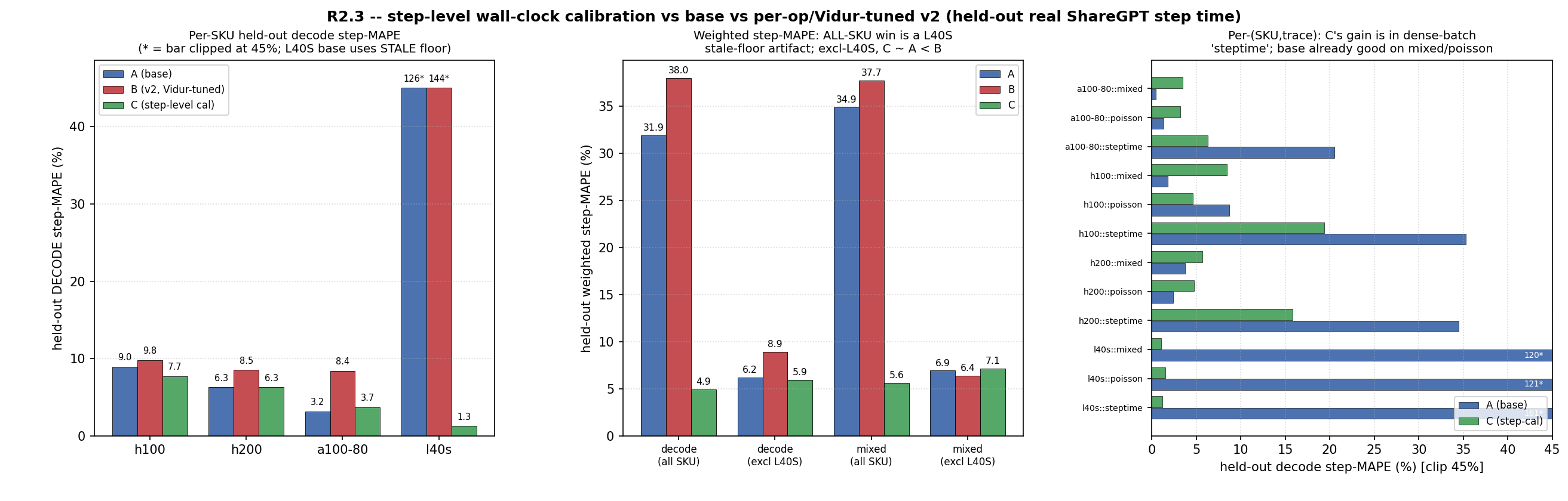
R2.3 held-out real ShareGPT step-MAPE. Left: per-SKU decode A/B/C (L40S base clipped at 45% — its shipped floor was the stale generate-proto value, since corrected (3149c31)). Middle: weighted decode/mixed, all-SKU vs excl-L40S — the headline all-SKU win (A 31.9→C 4.9) is dominated by C FIXING the stale L40S floor; excl-L40S, C≈A<B. Right: per-(SKU,trace) — C's gain is concentrated in the dense-batch 'steptime' traces (h100 35.3→19.4, a100-80 20.5→6.3), while base is already accurate on mixed/poisson. Source: results/blueprint_exp/R2_3_steplevel_cal.json (experiments/blueprint_R2_3.py).
2.6 'Online learning' is retired — the honest claim is ADAPT-ONLY (E1.19)
An earlier framing called the host floor S(N) 'online learning'. E1.19 settled it on real vLLM Poisson traces with four arms: STATIC (shipped), ORACLE-STATIC (best constant in hindsight), ONLINE-frozen (learn-then-deploy, frozen at the boundary), and a diagnostic continuously-adapting arm.
ADAPT-ONLY: on a stationary trace, frozen-online does NOT beat one-time calibration (gaps 0.22/0.43/0.21pp, online wins 1 of 3, within noise). It helps ONLY under shift: post-shift MAPE static 2.58% vs online 0.43%, adapting within 26 steps. The continuously-adapting arm flattered online via peeking. The phrase 'online learning' is retired. Source: E1_19_learner.json.
2.7 Accuracy — where it is strong and where it is weak
Decode is strong, prefill is weak, and round 1 localised it. On Vidur GT (A100, 18,601 cells): decode 6.2% / prefill 22.8% / agg 8.5%; the isolated fix moves prefill to 17.3% (E1.1). Cross-SKU prefill after fixes (E1.21): A100 5.81%, H100 6.70%, H200 7.49% (within 2× of home), but L40S 33.2% (the documented proxy SKU). On transfer (E2.1): decode 6.1/5.9/7.4%, prefill 23.0/30.7/32.5%.
E1.22 builds the per-cell error atlas; E1.23 runs the head-to-head vs re-implemented GenZ/LLM-Viewer/LIMINAL-style baselines on our cells across four SKUs, so the roofline comparison is measured, not asserted (E1_22.json, E1_23.json).
3. Part 2 — the utility (the predictor improves real systems)
Part 1 builds a predictor; Part 2 asks the harder question — does it help? Every system below ships its own (usually profiled) latency model. The test: does swapping in our profiling-free predictor at the hook measurably improve the decision? Round 1 turned this from narrated into measured.
3.1 Vidur cross-GPU transfer — THE decisive win (E2.1)
Vidur is a serving simulator whose accuracy rests on a random forest trained on one GPU's profiling. Its honest weakness: no profile for an unseen GPU. The experiment: train the RF on home A100, then have RF-verbatim, RF spec-scaled, and OURS predict on unseen H100/H200, scored against Vidur's own profiled GT there.
| Cell | RF spec-scaled | RF verbatim | OURS | OURS decode | Verdict |
|---|---|---|---|---|---|
| HOME A100 | 1.14% | 1.14% | 8.51% | 6.11% | RF wins |
| UNSEEN H100 | 11.38% | 88.14% | 7.28% | 5.89% | OURS 1.56× |
| UNSEEN H200 | 10.23% | 134.51% | 8.74% | 7.38% | OURS 1.17× |
Three honest reads. (1) On home A100 the RF is far more accurate (1.14% vs 8.51%); we win on cost/coverage (E2.5: 0.001s/0 rows vs ~158s/44k rows), not accuracy. (2) RF-verbatim off-home is useless (88%/135%). (3) Even the charitable spec-scaled RF loses to us on both unseen cards: 1.56×/1.17× (all), 1.87×/1.34× (decode). Decode-driven; our prefill is weaker on unseen cards (30.7%/32.5%). This is the Part-2 number that was open in v1 and is now in hand. Source: transfer_2x2.json.
3.2 Honest SKU-ranking — the tie-aware re-score (E2.6)
An earlier result claimed 100% top-1 SKU ranking. E2.6 found the artifact: H100/H200 share an identical 989-TF peak and η̄=0.75, so at M≥512 their predicted times are EXACTLY equal — a tie that sorted() broke by insertion order and scored as a hit. Tie-aware re-score: 72 correct / 0 wrong / 6 unbroken ties over 78 pairs = 92.3% tie-aware, 100% when it decides. The large-M compute crossover stays an honest tie (the signal is off-datasheet, needs measured data). Source: E2_6.json.
3.3 DistServe — matching a profiled model with zero profiling
DistServe ships a profiled latency model. On its own GPU/model (OPT-13B/A100), our fit-free predictor reaches 1.78% step-MAPE vs DistServe's 2.27% — matching, slightly beating, a profiled model with zero profiling. The clean accuracy-parity datapoint.
3.4 QLM — estimator fixed, SLO result honestly MIXED (E2.3)
QLM's EDF ordering depends on a waiting-time estimator. Swapping its native scalar estimator for ours is a large standalone accuracy win (111–123% → ~1%, plus a hardware axis). The honest question: does that translate into live SLO attainment? E2.3 ran the contended concurrent-executor test the prior null could not.
3.5 Power-aware scheduling — the two-paper bridge (E2.8)
This links the freq work (Part 1) to the utility work (Part 2). Prior power-aware schedulers treat frequency as a commanded set-point with a cap-/M-blind peak. None models the involuntary droop of the DELIVERED clock under a cap as a function of M. We measured it on the RTX 5090: the 400 W-vs-575 W penalty is ~0% at small M (0.08% @M=64, 0.99% @M=1024) and rises (7.7% @M=4096, 10.7% @M=16384).
3.6 Sarathi chunk-sizing — +30.7% throughput at matched SLO (E2.9)
Sarathi's chunked-prefill scheduler exposes one tunable — the chunk budget — trading co-scheduled step latency (TBT) against throughput. Picking the budget that meets a TBT SLO at max throughput normally needs an offline profiling sweep. The claim: our fit-free predictor picks it with zero profiling and beats the static default.
3.7 Splitwise & the in-flight end-to-end run (E2.10)
Splitwise is a coverage case: our predictor supplies per-phase costs the profiled model cannot off-home, so the contribution is coverage, not a head-to-head metric. The one remaining utility experiment is E2.10 — a fully end-to-end live vLLM serving run closing the loop from predictor to served-trace metrics. It is still in the PACE queue, marked IN-FLIGHT; its numbers are deliberately not stated because they do not yet exist in a result file.
3.8 The Part-2 abstract figure — every integration, color-coded by claim type (E2.7)
The abstract sentence — 'on N real systems, swapping in our predictor improves X by Y%' — is backed by exactly this table, stating each integration honestly including where we lose, where it is coverage-only, and where it is mixed. The claim type is the discipline. Every row cites its file.
| System | What we replace | Claim type | Honest outcome |
|---|---|---|---|
| Vidur | profiled RF step model | transfer accuracy | unseen 1.56×/1.17×; home RF wins (E2.1) |
| Vidur | SKU-ranking decision | decision quality | 92.3% tie-aware; 100% when it decides (E2.6) |
| DistServe | profiled p/d latency model | accuracy parity | 1.78% vs 2.27%, zero profiling |
| QLM | native waiting-time estimator | estimate accuracy | 111–123% → ~1% standalone (E2.3) |
| QLM | same estimator, live SLO | SLO — MIXED | +4.25pp@40, −26.0pp@80 (E2.3) |
| Power-aware | cap-/M-blind peak | decision quality | +10.5% makespan; oracle 6/6 (E2.8) |
| Sarathi-Serve | static chunk-budget default | throughput @ SLO | Spearman 1.0; +30.7% @SLO (E2.9) |
| Splitwise | per-phase placement cost | coverage | coverage off-home, not a metric delta |
| End-to-end live vLLM | full serving loop | IN-FLIGHT | E2.10 in PACE queue; not yet reduced |
Read this as the abstract: a genuine measured improvement on four head-to-head systems, an honest mixed result on QLM SLO, a coverage-only capability on Splitwise, and one still running (E2.10). Nothing is claimed beyond its file.
4. Honest status — the scorecard after round 1
The same questions, re-scored. Big movers: Q-vidur cross-GPU NOT-DONE→SOLID (E2.1); Q-twofactors and Q-L2 firmed up (E1.13, E1.15, E1.3c); Q-online resolved to ADAPT-ONLY; the metric-divergence lesson (E1.16) recorded as PARTIAL with an explanation.
| Question / item | Status | One-line basis (file) |
|---|---|---|
| PART 1 — THE PREDICTOR | ||
| Q-freq A (clock droop) | SOLID | f_clk isolated, n=5; Blackwell 54.4% (E1_5/E1_10) |
| Q-freq B (GEMM slows under cap) | PARTIAL | L40S −15.6%; clock-norm flattens; PACE denied lock (E1_8) |
| Q-freq (cap→clock→decline) | PARTIAL | cap→clock proven; decline lock deferred (E1_9) |
| Q-smfill (cluster cap) | SOLID | 112=7×16 GPC closed form (E1_11) |
| Q-smfill (Blackwell) | SOLID | sm120 = Ampere-style, no clusters (E1_12) |
| Q-twofactors (active ⊥ duty) | SOLID | single SoT module reconciles both (E1_13) |
| Q-twofactors (η_duty law) | IN-FLIGHT | denser-M law: 2/4 jobs, held partial (E1.14) |
| Q-twofactors (L40S CV) | SOLID | 0.425, CV→1.8% (n=32) (E1_15) |
| Q-L2 (param-only memory) | SOLID | global law, 3 SKUs, 4.59%; L40S blocked (E1_3c) |
| Q-L2 (in predictor) / metric divergence | PARTIAL | v2 helps Vidur, hurts real wall-clock (E1_16) |
| Q-L2 (bench-vs-engine) | PARTIAL | law ≠ engine kernels, 42.3% gap (E1_17) |
| Q-overlap (α derived) | SOLID | nsys reduced, α≈1 eager (E1_4) |
| Q-online (online learning?) | ADAPT-ONLY | ≈ static stationary; wins under shift (E1_19) |
| Q-count (only three?) | SOLID | ≥7 terms; ΔMAPE ledger (E1_20) |
| Q-count (light/KV dominates) | SOLID | 81% residual; per-kernel 16.2%, est→6.6% |
| Q-acc (decode) | SOLID | 0.8–3.7% real; 5.9–7.4% unseen Hopper |
| Q-acc (prefill) | PARTIAL | cross-SKU 5.8/6.7/7.5%; L40S 33% (E1_21) |
| Q-acc (vs prior models) | SOLID | vs 3 baselines, 4 SKUs (E1_23) |
| PART 2 — THE UTILITY | ||
| Q-vidur-rf (home MAPE) | SOLID | RF wins home; we win cost (E2.1/E2.5) |
| Q-vidur-rf (cross-GPU) | SOLID — WIN | unseen 1.56×/1.17×; RF-verbatim 88–135% |
| Q-vidur-decision (rank SKU) | SOLID | tie-aware 92.3%; Hopper honest tie (E2_6) |
| Q-qlm (estimate accuracy) | SOLID | 111–123% → ~1% (E2.3) |
| Q-qlm (SLO attainment) | MIXED | +4.2pp@40, −26pp@80 (E2_3) |
| Q-abstract (power-aware) | SOLID | +10.5% makespan; oracle 6/6 (E2_8) |
| Q-abstract (Sarathi chunk) | SOLID | Spearman 1.0; +30.7% @SLO (E2_9) |
| Q-abstract (DistServe / Splitwise) | SOLID | DistServe parity; Splitwise coverage |
| Q-abstract (end-to-end live) | IN-FLIGHT | E2.10 in PACE queue; not yet reduced |
5. What comes next
After round 1 the open items are few and specific, in two buckets. First, queued experiments: E1.14 (η_duty law on a denser M ladder, 2/4 jobs done) and E2.10 (end-to-end live vLLM). Both dispatched, not reduced — marked in-flight, numbers deliberately absent.
Second, the modeled-not-validated closes and the half-closed chain. E1.1c ESTIMATES prefill → ~6.6%; the honest next step is the full-step re-run with the per-kernel model swapped in. The cap→clock→decline chain is half-closed (cap→clock proven; PACE denied the L40S lock, E1.8), so the decisive lock must run on a lab card (E1.9). The L2 law's L40S cell is blocked and should be re-collected. And E1.16 leaves a genuine modeling question — integrate the factors to improve the Vidur target WITHOUT degrading real wall-clock — not a missing run.
None change the honest verdict. The decode predictor is real, accurate, and useful; the cross-GPU transfer win (E2.1) is the decisive Part-2 number, in hand; power-aware and Sarathi are clean wins; QLM SLO is honestly mixed; prefill, the v2 integration, and the cap→decline lock are the named, bounded gaps. What remains is exactly what moves the last PARTIAL/IN-FLIGHT rows to solid — enumerated, not hand-waved.